16.4. Select and Train a Model

16.4.1. Splitting data into Train and Test

import numpy as np
from sklearn.model_selection import train_test_split
X, y = np.arange(10).reshape((5, 2)), [0, 1, 0, 0, 1]
X
list(y)
# X -- feature
# y -- label

[0, 1, 0, 0, 1]

X_train, X_test, y_train, y_test = train_test_split(X, y, test_size=0.2)

X_train

y_train

X_test

y_test

[1]

X_train, X_test, y_train, y_test = train_test_split(
    X, y, test_size=0.40, random_state=43)

X_train

y_train

X_test

y_test

[0, 0]

X_train, X_test, y_train, y_test = train_test_split(
    X, y, test_size=0.33, random_state=42)

X_train

y_train

X_test

y_test

[1, 1]

import random
X_train, X_test, y_train, y_test = train_test_split(
    X, y, test_size=0.33, random_state=random.randint(1, 10000))

X_train

y_train

X_test

y_test

[0, 1]

import random
X_train, X_test, y_train, y_test = train_test_split(
    X, y, test_size=0.33, random_state=random.randint(1, 10000))

X_train

y_train

X_test

y_test

[0, 0]

import pandas as pd
from sklearn import datasets, linear_model
from sklearn.model_selection import train_test_split
from matplotlib import pyplot as plt

diabetes = datasets.load_diabetes()
diabetes.data.shape

feature_names = diabetes.feature_names
feature_names

['age', 'sex', 'bmi', 'bp', 's1', 's2', 's3', 's4', 's5', 's6']

df = pd.DataFrame(diabetes.data, columns=feature_names)
y = diabetes.target
df
y
df.shape

(442, 10)

import random
X_train, X_test, y_train, y_test = train_test_split(df, y, test_size=0.2, random_state=random.randint(1, 10000))

X_train

y_train

X_test

y_test

array([292., 262., 321.,  94., 126.,  65., 155., 144., 277., 182., 160.,
       173., 103., 178.,  60., 214.,  59.,  95., 219., 179.,  68., 114.,
        84.,  85., 230., 128.,  69.,  51.,  96.,  74., 210.,  77.,  25.,
        39., 220.,  63., 174.,  81., 180.,  53.,  51., 257.,  87., 118.,
        74.,  60., 195.,  40.,  94., 181., 259.,  70., 104., 158.,  88.,
        97., 202.,  44.,  65., 283., 150.,  85., 158., 127.,  48., 196.,
        84.,  64., 170., 274.,  93.,  63., 332.,  71.,  31., 162., 189.,
       139.,  66., 129., 214.,  65., 233.,  65., 202., 206., 115., 109.,
        88.])

X_train.shape

len(y_train)

X_test.shape

len(y_test)

89

16.4.2. Linear Regression Example

• To predict a numerical value

import numpy as np
from sklearn.linear_model import LinearRegression
X = np.array([[1, 1], [1, 2], [2, 2], [2, 3]])
# y = 1 * x_0 + 2 * x_1 + 3
y = np.dot(X, np.array([1, 2])) + 3
reg = LinearRegression().fit(X, y)
reg.score(X, y)

reg.coef_

reg.intercept_ 

# y = mx + b

reg.predict(np.array([[3, 5]]))

array([16.])

import numpy as np
import pandas as pd
from sklearn.model_selection import train_test_split
from sklearn.linear_model import LinearRegression
from sklearn import metrics
from sklearn.metrics import r2_score

dataset=pd.read_csv('Salary_Data.csv')
dataset.head()
dataset.shape
dataset

	YearsExperience	Salary
0	1.1	39343.0
1	1.3	46205.0
2	1.5	37731.0
3	2.0	43525.0
4	2.2	39891.0
5	2.9	56642.0
6	3.0	60150.0
7	3.2	54445.0
8	3.2	64445.0
9	3.7	57189.0
10	3.9	63218.0
11	4.0	55794.0
12	4.0	56957.0
13	4.1	57081.0
14	4.5	61111.0
15	4.9	67938.0
16	5.1	66029.0
17	5.3	83088.0
18	5.9	81363.0
19	6.0	93940.0
20	6.8	91738.0
21	7.1	98273.0
22	7.9	101302.0
23	8.2	113812.0
24	8.7	109431.0
25	9.0	105582.0
26	9.5	116969.0
27	9.6	112635.0
28	10.3	122391.0
29	10.5	121872.0

16.4.2.1. Selecting the data

X = dataset.iloc[:, :-1].values
y = dataset.iloc[:, 1].values
X
y

array([ 39343.,  46205.,  37731.,  43525.,  39891.,  56642.,  60150.,
        54445.,  64445.,  57189.,  63218.,  55794.,  56957.,  57081.,
        61111.,  67938.,  66029.,  83088.,  81363.,  93940.,  91738.,
        98273., 101302., 113812., 109431., 105582., 116969., 112635.,
       122391., 121872.])

16.4.2.2. Split the data

from sklearn.model_selection import train_test_split
X_train, X_test, y_train, y_test=train_test_split(X, y, test_size=0.20)

16.4.2.3. Train and Test

from sklearn.linear_model import LinearRegression
regressor=LinearRegression()
regressor.fit(X_train,y_train)
y_pred=regressor.predict(X_test)
y_pred
y_test
metrics.mean_squared_error(y_test, y_pred, squared=False)

/home/mkzia/anaconda3/envs/eas503book/lib/python3.12/site-packages/sklearn/metrics/_regression.py:492: FutureWarning: 'squared' is deprecated in version 1.4 and will be removed in 1.6. To calculate the root mean squared error, use the function'root_mean_squared_error'.
  warnings.warn(

np.float64(5826.62642968907)

r2_score(y_test, y_pred)
regressor.coef_
regressor.intercept_

np.float64(25464.3071225343)

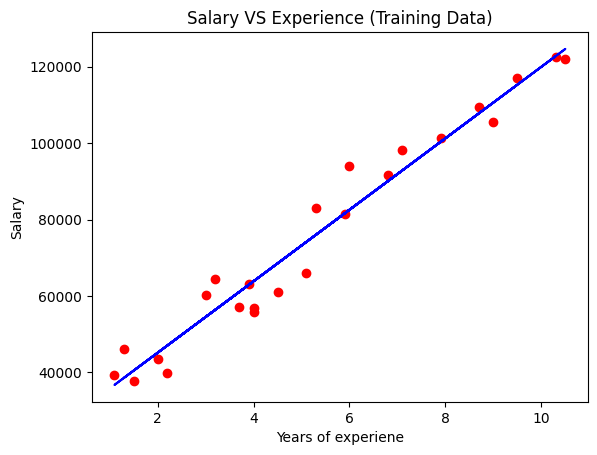
plt.scatter(X_train,y_train,color='red')
plt.plot(X_train,regressor.predict(X_train),color='blue')
plt.title('Salary VS Experience (Training Data)')
plt.xlabel('Years of experiene')
plt.ylabel('Salary')
plt.show()

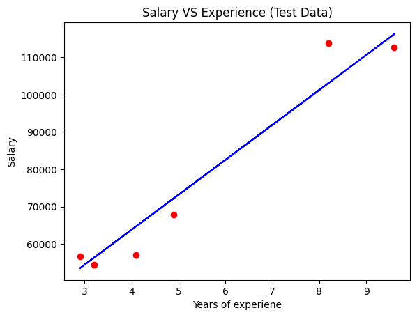
plt.scatter(X_test,y_test,color='red')
plt.plot(X_test,regressor.predict(X_test),color='blue')
plt.title('Salary VS Experience (Test Data)');
plt.xlabel('Years of experiene');
plt.ylabel('Salary');
plt.show()

16.4.2.4. Apply DecisionTreeRegressor

• Decision Trees are good for finding complex nonlinear relationships

X = dataset.iloc[:, :-1].values
y = dataset.iloc[:, 1].values
from sklearn.model_selection import train_test_split
X_train, X_test, y_train, y_test=train_test_split(X, y, test_size=0.20)

from sklearn.tree import DecisionTreeRegressor
regressor=DecisionTreeRegressor()
regressor.fit(X_train,y_train)
y_pred=regressor.predict(X_test)
y_pred
y_test
metrics.mean_squared_error(y_test, y_pred, squared=False)

/home/mkzia/anaconda3/envs/eas503book/lib/python3.12/site-packages/sklearn/metrics/_regression.py:492: FutureWarning: 'squared' is deprecated in version 1.4 and will be removed in 1.6. To calculate the root mean squared error, use the function'root_mean_squared_error'.
  warnings.warn(

np.float64(6834.143094297437)

16.4.2.5. Cross-Validation

from sklearn.pipeline import make_pipeline
X = dataset.iloc[:, :-1].values
y = dataset.iloc[:, 1].values
preprocessing = make_pipeline(StandardScaler())
reg_pipeline = make_pipeline(preprocessing, LinearRegression())
reg_pipeline.fit(X, y)
y_pred=reg_pipeline.predict(X)
metrics.mean_squared_error(y, pred, squared=False)
from sklearn.model_selection import cross_val_score
reg_rmses = cross_val_score(reg_pipeline, X, y, scoring="neg_root_mean_squared_error", cv=10)

---------------------------------------------------------------------------
NameError                                 Traceback (most recent call last)
Cell In[20], line 4
      2 X = dataset.iloc[:, :-1].values
      3 y = dataset.iloc[:, 1].values
----> 4 preprocessing = make_pipeline(StandardScaler())
      5 reg_pipeline = make_pipeline(preprocessing, LinearRegression())
      6 reg_pipeline.fit(X, y)

NameError: name 'StandardScaler' is not defined

from sklearn.pipeline import make_pipeline
X = dataset.iloc[:, :-1].values
y = dataset.iloc[:, 1].values
preprocessing = make_pipeline(StandardScaler())
tree_pipeline = make_pipeline(preprocessing, DecisionTreeRegressor())
tree_rmses = cross_val_score(tree_pipeline, X, y, scoring="neg_root_mean_squared_error", cv=10)
pd.Series(tree_rmses).describe()

---------------------------------------------------------------------------
NameError                                 Traceback (most recent call last)
Cell In[21], line 4
      2 X = dataset.iloc[:, :-1].values
      3 y = dataset.iloc[:, 1].values
----> 4 preprocessing = make_pipeline(StandardScaler())
      5 tree_pipeline = make_pipeline(preprocessing, DecisionTreeRegressor())
      6 tree_rmses = cross_val_score(tree_pipeline, X, y, scoring="neg_root_mean_squared_error", cv=10)

NameError: name 'StandardScaler' is not defined

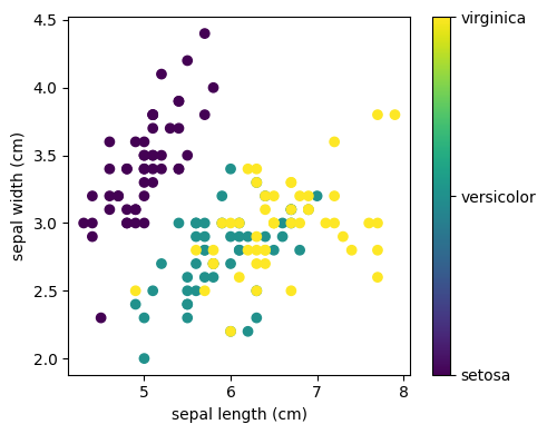
16.4.3. Classification Example

from sklearn.datasets import load_iris
from sklearn.model_selection import train_test_split
from sklearn import metrics
from sklearn.naive_bayes import GaussianNB
# Load the data
from sklearn.datasets import load_iris
iris = load_iris()

from matplotlib import pyplot as plt

# The indices of the features that we are plotting
x_index = 0
y_index = 1

# this formatter will label the colorbar with the correct target names
formatter = plt.FuncFormatter(lambda i, *args: iris.target_names[int(i)])

plt.figure(figsize=(5, 4))
plt.scatter(iris.data[:, x_index], iris.data[:, y_index], c=iris.target)
plt.colorbar(ticks=[0, 1, 2], format=formatter)
plt.xlabel(iris.feature_names[x_index])
plt.ylabel(iris.feature_names[y_index])

plt.tight_layout()
plt.show()

X = iris.data
Y = iris.target
X_train, X_test, y_train, y_test=train_test_split(X, Y, test_size=0.2, random_state=0)

gnb = GaussianNB()
gnb.fit(X_train, y_train)
y_pred = gnb.predict(X_test)
100*metrics.accuracy_score(y_test, y_pred)

96.66666666666667