
16.3. Preprocessing data#
16.3.1. Standardization, or mean removal and variance scaling#
Standardization of datasets is a common requirement for many machine learning estimators implemented in scikit-learn; they might behave badly if the individual features do not more or less look like standard normally distributed data: Gaussian with zero mean and unit variance.
In practice we often ignore the shape of the distribution and just transform the data to center it by removing the mean value of each feature, then scale it by dividing non-constant features by their standard deviation.
from IPython.display import display
from sklearn.datasets import load_iris
iris_dataset = load_iris()
from sklearn import preprocessing
import numpy as np
import pandas as pd
X_train = np.array([[ 1., -1.,  2.],
                    [ 2.,  0.,  0.],
                    [ 0.,  1., -1.]])

df = pd.DataFrame(X_train)
display(df)

X_scaled = preprocessing.scale(df)

X_scaled

#rows are different patients/subjects/flowers
# columns are various features of the patients/subjects/flowers
| 0 | 1 | 2 | |
|---|---|---|---|
| 0 | 1.0 | -1.0 | 2.0 |
| 1 | 2.0 | 0.0 | 0.0 |
| 2 | 0.0 | 1.0 | -1.0 |
array([[ 0.        , -1.22474487,  1.33630621],
       [ 1.22474487,  0.        , -0.26726124],
       [-1.22474487,  1.22474487, -1.06904497]])
df.describe()
| 0 | 1 | 2 | |
|---|---|---|---|
| count | 3.0 | 3.0 | 3.000000 |
| mean | 1.0 | 0.0 | 0.333333 |
| std | 1.0 | 1.0 | 1.527525 |
| min | 0.0 | -1.0 | -1.000000 |
| 25% | 0.5 | -0.5 | -0.500000 |
| 50% | 1.0 | 0.0 | 0.000000 |
| 75% | 1.5 | 0.5 | 1.000000 |
| max | 2.0 | 1.0 | 2.000000 |
idata = iris_dataset.data
id_scaled = preprocessing.scale(idata)
idata.mean(axis=0)
id_scaled.mean(axis=0)
id_scaled.var(axis=0)
array([1., 1., 1., 1.])
X_train.mean(axis=0)
X_scaled.mean(axis=0)
array([0., 0., 0.])
X_scaled.std(axis=0)
X_scaled.mean(axis=1)
X_scaled.std(axis=1)
array([1.04587533, 0.64957343, 1.11980724])
16.3.2. Can save scaling and apply to testing data#
Never ever apply any preprocessing or any other step on all your data and then train. This will lead to Data Leakage!
scaler = preprocessing.StandardScaler().fit(X_train)
scaler
scaler.transform(X_train)
array([[ 0.        , -1.22474487,  1.33630621],
       [ 1.22474487,  0.        , -0.26726124],
       [-1.22474487,  1.22474487, -1.06904497]])
Note
Be careful about data leakage https://www.atoti.io/articles/what-is-data-leakage-and-how-to-mitigate-it/
X_test = [[-1., 1., 0.]]
scaler.transform(X_test)
array([[-2.44948974, 1.22474487, -0.26726124]])
16.3.3. Scaling features to a range#
X_train = np.array([[ 1., -1.,  2.],
                    [ 2.,  0.,  0.],
                    [ 0.,  1., -1.]])

min_max_scaler = preprocessing.MinMaxScaler()
X_train_minmax = min_max_scaler.fit_transform(X_train)
X_train_minmax
array([[0.5       , 0.        , 1.        ],
       [1.        , 0.5       , 0.33333333],
       [0.        , 1.        , 0.        ]])
X_test = np.array([[-3., -1.,  4.]])
X_test_minmax = min_max_scaler.transform(X_test)
X_test_minmax
array([[-1.5 , 0. , 1.66666667]])
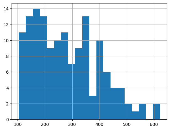
16.3.4. Pre-processing data - Non-linear transformation#
This is a very silly example, but just demonstrating usage.
import pandas as pd
%matplotlib inline
df = pd.read_csv('international-airline-passengers.csv')
display(df)
| date | passengers | |
|---|---|---|
| 0 | 1949-01 | 112.0 |
| 1 | 1949-02 | 118.0 |
| 2 | 1949-03 | 132.0 |
| 3 | 1949-04 | 129.0 |
| 4 | 1949-05 | 121.0 |
| ... | ... | ... |
| 140 | 1960-09 | 508.0 |
| 141 | 1960-10 | 461.0 |
| 142 | 1960-11 | 390.0 |
| 143 | 1960-12 | 432.0 |
| 144 | International airline passengers: monthly tota... | NaN |
145 rows × 2 columns
df['passengers'].hist(bins=20)
<Axes: >
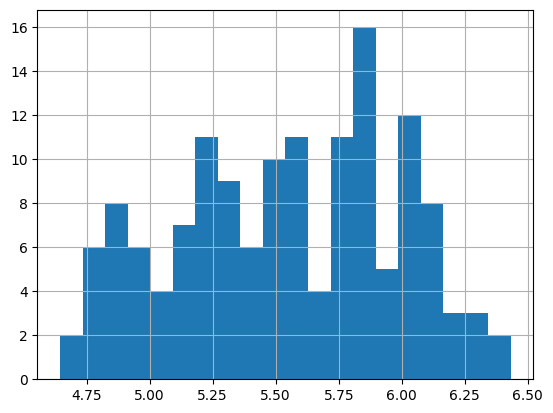
import numpy as np
df['passengers'] = np.log(df['passengers'])
df['passengers'].hist(bins=20)
<Axes: >
16.3.5. Normalization#
from sklearn import preprocessing
X = [[ 1., -1.,  2.],
     [ 2.,  0.,  0.],
     [ 0.,  1., -1.]]
X_normalized = preprocessing.normalize(X, norm='l1')

X_normalized
# http://www.chioka.in/differences-between-the-l1-norm-and-the-l2-norm-least-absolute-deviations-and-least-squares/
array([[ 0.25, -0.25,  0.5 ],
       [ 1.  ,  0.  ,  0.  ],
       [ 0.  ,  0.5 , -0.5 ]])
16.3.5.1. Can save the normalization for future use#
normalizer = preprocessing.Normalizer().fit(X)  # fit does nothing
normalizer.transform(X)
array([[ 0.40824829, -0.40824829,  0.81649658],
       [ 1.        ,  0.        ,  0.        ],
       [ 0.        ,  0.70710678, -0.70710678]])
normalizer.transform([[2., 1., 0.]])
array([[0.89442719, 0.4472136 , 0. ]])
16.3.6. Preprocessing data - Encoding#
from sklearn import preprocessing
enc = preprocessing.OrdinalEncoder()
X = [['male', 'from US', 'uses Safari'],
     ['female', 'from Europe', 'uses Firefox']]
enc.fit(X)
OrdinalEncoder()In a Jupyter environment, please rerun this cell to show the HTML representation or trust the notebook.
On GitHub, the HTML representation is unable to render, please try loading this page with nbviewer.org.
OrdinalEncoder()
enc.transform([['female', 'from US', 'uses Safari']])
array([[0., 1., 1.]])
enc.transform([['male', 'from Europe', 'uses Safari']])
array([[1., 0., 1.]])
enc.transform([['female', 'from Europe', 'uses Firefox']])
array([[0., 0., 0.]])
16.3.6.1. One Hot Encoder#
genders = ['female', 'male']
locations = ['from Africa', 'from Asia', 'from Europe', 'from US']
browsers = ['uses Chrome', 'uses Firefox', 'uses IE', 'uses Safari']
enc = preprocessing.OneHotEncoder(categories=[genders, locations, browsers])
X = [['male', 'from US', 'uses Safari'], ['female', 'from Europe', 'uses Firefox']]
enc.fit(X)
enc.categories_
[array(['female', 'male'], dtype=object),
 array(['from Africa', 'from Asia', 'from Europe', 'from US'], dtype=object),
 array(['uses Chrome', 'uses Firefox', 'uses IE', 'uses Safari'],
       dtype=object)]
enc.transform([['male', 'from US', 'uses Safari']])
<1x10 sparse matrix of type '<class 'numpy.float64'>'
	with 3 stored elements in Compressed Sparse Row format>
tmp = enc.transform([['female', 'from Asia', 'uses Chrome'],
                    ['male', 'from Europe', 'uses Safari']]).toarray()
tmp
array([[1., 0., 0., 1., 0., 0., 1., 0., 0., 0.],
       [0., 1., 0., 0., 1., 0., 0., 0., 0., 1.]])
16.3.7. Discretization#
Discretization (otherwise known as quantization or binning) provides a way to partition continuous features into discrete values. Certain datasets with continuous features may benefit from discretization, because discretization can transform the dataset of continuous attributes to one with only nominal attributes.
One-hot encoded discretized features can make a model more expressive, while maintaining interpretability. For instance, pre-processing with a discretizer can introduce nonlinearity to linear models.
X = np.array([[ -3., 5., 15 ],
              [  0., 6., 14 ],
              [  6., 3., 11 ]])
est = preprocessing.KBinsDiscretizer(n_bins=[3, 2, 4], encode='ordinal').fit(X)
est.transform(X)
array([[0., 1., 3.],
       [1., 1., 2.],
       [2., 0., 0.]])
16.3.8. Univariate feature imputation#
Impute missing values
import numpy as np
from sklearn.impute import SimpleImputer
imp = SimpleImputer(missing_values=np.nan, strategy='mean')
orig_data = [[1, 2],
         [np.nan, 3],
         [7, 6]]
imp.fit(orig_data)
imp.transform(orig_data)
array([[1., 2.],
       [4., 3.],
       [7., 6.]])
X = [[np.nan, 2],
     [6, np.nan],
     [7, 6]]
print(imp.transform(X))
[[4.         2.        ]
 [6.         3.66666667]
 [7.         6.        ]]
import pandas as pd
df = pd.DataFrame([["a", "x"],
                   [np.nan, "w"],
                   ["a", np.nan],
                   ["b", "y"]], dtype="category")

imp = SimpleImputer(strategy="most_frequent")
print(imp.fit_transform(df))
[['a' 'x']
 ['a' 'w']
 ['a' 'w']
 ['b' 'y']]
import pandas as pd
df = pd.DataFrame([["a", "x"],
                   [np.nan, "y"],
                   ["c", np.nan],
                   ["b", "y"]], dtype="category")

imp = SimpleImputer(strategy="most_frequent")
print(imp.fit_transform(df))
[['a' 'x']
 ['a' 'y']
 ['c' 'y']
 ['b' 'y']]
16.3.9. Review Book Examples#
https://en.wikipedia.org/wiki/Correlation#/media/File:Correlation_examples2.svg
https://scikit-learn.org/stable/auto_examples/miscellaneous/plot_pipeline_display.html