
16.5. Feature Selection and Evaluation#
16.5.1. PCA#
from IPython.core.interactiveshell import InteractiveShell
InteractiveShell.ast_node_interactivity = "all"
import numpy as np
from scipy import signal
import matplotlib.pyplot as plt
%matplotlib inline
np.random.seed = 1
N = 1000
fs = 500
w = np.arange(1,N+1) * 2 * np.pi/fs
t = np.arange(1,N+1)/fs
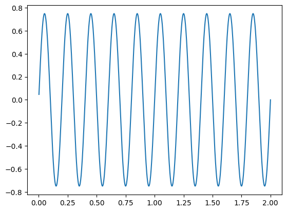
x = 0.75 * np.sin(w*5)
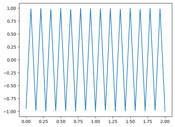
y = signal.sawtooth(w*7, 0.5)
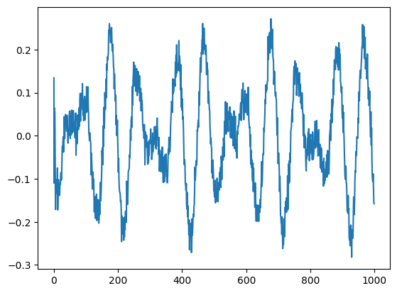
d1 = 0.5*y + 0.5*x + 0.1*np.random.rand(1,N)
d2 = 0.2*y + 0.75*x + 0.15*np.random.rand(1,N)
d3 = 0.7*y + 0.25*x + 0.1*np.random.rand(1,N)
d4 = -0.5*y + 0.4*x + 0.2*np.random.rand(1,N)
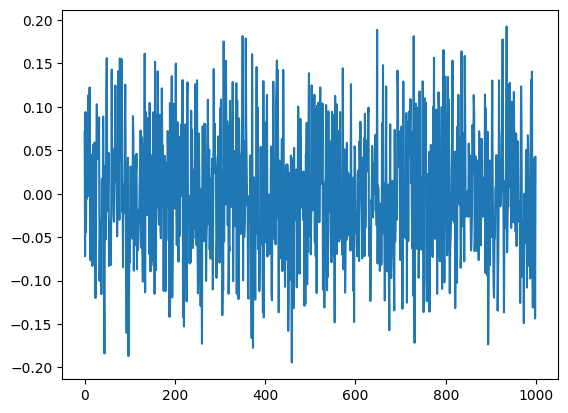
d5 = 0.6*np.random.rand(1,N)
d1 = d1 - d1.mean()
d2 = d2 - d2.mean()
d3 = d3 - d3.mean()
d4 = d4 - d4.mean()
d5 = d5 - d5.mean()
plt.plot(d1.transpose())
[<matplotlib.lines.Line2D at 0x714c506d9580>]

plt.plot(t, x)
[<matplotlib.lines.Line2D at 0x714c5074d5e0>]
plt.plot(t, y)
[<matplotlib.lines.Line2D at 0x714c4e47dcd0>]
import numpy as np
X = np.array([d1[0], d2[0], d3[0], d4[0], d5[0]])
X
X.shape
array([[-0.48495245, -0.39938569, -0.37206311, ..., -0.48925259,
        -0.53864604, -0.46576956],
       [-0.14503941, -0.17831242, -0.07159727, ..., -0.21973243,
        -0.16437217, -0.13974172],
       [-0.66217825, -0.58594889, -0.53933795, ..., -0.69347791,
        -0.64016754, -0.70446435],
       [ 0.46736157,  0.44175446,  0.42081984, ...,  0.37586476,
         0.50996614,  0.42273577],
       [ 0.28984768, -0.08849879, -0.2152407 , ..., -0.12974106,
         0.01963351,  0.16215695]], shape=(5, 1000))
(5, 1000)
U,S,V = np.linalg.svd(X)
S
array([20.90143292, 14.22773131, 5.32587574, 1.4730656 , 0.99739728])
for i in range(5):
    V[:,i] = V[:,i] * np.sqrt(S[i])
eigen = S**2
eigen
array([436.86989819, 202.4283383 ,  28.36495235,   2.16992227,
         0.99480133])
eigen = eigen/N
eigen = eigen/sum(eigen)
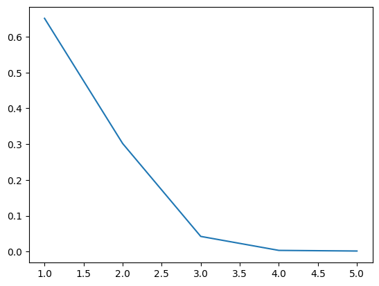
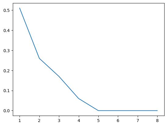
16.5.1.1. Scree plot#
Gives the measure of the associated principal component’s importance with regards to how much of the total information it represents.
plt.plot(range(1,6), eigen)
[<matplotlib.lines.Line2D at 0x714c4e43be30>]
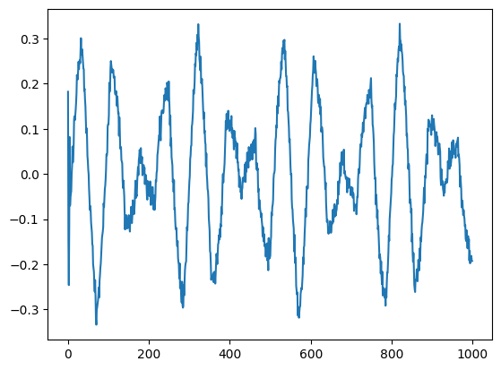
plt.plot(V[:,0])
plt.show()
[<matplotlib.lines.Line2D at 0x714c4e499760>]
plt.plot(V[:,1])
plt.show()
[<matplotlib.lines.Line2D at 0x714c4db2bc20>]
plt.plot(V[:,2])
plt.show()
[<matplotlib.lines.Line2D at 0x714c4dba9010>]
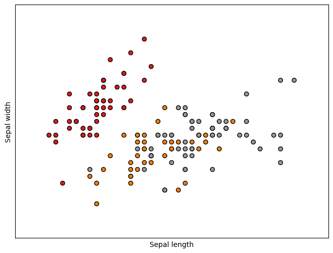
16.5.1.2. PCA on the IRIS Data#
import matplotlib.pyplot as plt
from mpl_toolkits.mplot3d import Axes3D
from sklearn import datasets
from sklearn.decomposition import PCA

# import some data to play with
iris = datasets.load_iris()
X = iris.data[:, :2]  # we only take the first two features.
y = iris.target

x_min, x_max = X[:, 0].min() - .5, X[:, 0].max() + .5
y_min, y_max = X[:, 1].min() - .5, X[:, 1].max() + .5

plt.figure(2, figsize=(8, 6))
plt.clf()

# Plot the training points
plt.scatter(X[:, 0], X[:, 1], c=y, cmap=plt.cm.Set1,
            edgecolor='k')
plt.xlabel('Sepal length')
plt.ylabel('Sepal width')

plt.xlim(x_min, x_max)
plt.ylim(y_min, y_max)
plt.xticks(())
plt.yticks(())

# To getter a better understanding of interaction of the dimensions
# plot the first three PCA dimensions
fig = plt.figure(1, figsize=(8, 6))
ax = Axes3D(fig, elev=-150, azim=110)
X_reduced = PCA(n_components=3).fit_transform(iris.data)
ax.scatter(X_reduced[:, 0], X_reduced[:, 1], X_reduced[:, 2], c=y,
           cmap=plt.cm.Set1, edgecolor='k', s=40)
ax.set_title("First three PCA directions")
ax.set_xlabel("1st eigenvector")
ax.w_xaxis.set_ticklabels([])
ax.set_ylabel("2nd eigenvector")
ax.w_yaxis.set_ticklabels([])
ax.set_zlabel("3rd eigenvector")
ax.w_zaxis.set_ticklabels([])

plt.show()
<Figure size 800x600 with 0 Axes>
<matplotlib.collections.PathCollection at 0x714c4c980260>
Text(0.5, 0, 'Sepal length')
Text(0, 0.5, 'Sepal width')
(3.8, 8.4)
(1.5, 4.9)
([], [])
([], [])
<mpl_toolkits.mplot3d.art3d.Path3DCollection at 0x714c4cbe0770>
Text(0.5, 0.92, 'First three PCA directions')
Text(0.5, 0, '1st eigenvector')
---------------------------------------------------------------------------
AttributeError                            Traceback (most recent call last)
Cell In[13], line 37
     35 ax.set_title("First three PCA directions")
     36 ax.set_xlabel("1st eigenvector")
---> 37 ax.w_xaxis.set_ticklabels([])
     38 ax.set_ylabel("2nd eigenvector")
     39 ax.w_yaxis.set_ticklabels([])

AttributeError: 'Axes3D' object has no attribute 'w_xaxis'
<Figure size 800x600 with 0 Axes>
iris = datasets.load_iris()
X = iris.data[:50,:]
X2 = X +0.05*np.random.rand(50,4)
X_combined = np.zeros((50,8))
X_combined[:,0:4] = X
X_combined[:,4:] = X2
X_combined.mean(axis=0)
array([5.006     , 3.428     , 1.462     , 0.246     , 5.03265378,
       3.45142158, 1.4859936 , 0.2673384 ])
from sklearn import preprocessing
X_scaled = preprocessing.scale(X_combined)
X_combined.mean(axis=0)
array([5.006     , 3.428     , 1.462     , 0.246     , 5.03265378,
       3.45142158, 1.4859936 , 0.2673384 ])
U,S,V = np.linalg.svd(X_scaled)
S
array([14.27474011, 10.19852281,  8.1422001 ,  5.01659152,  0.72777529,
        0.39100058,  0.23198786,  0.15478182])
eigen = S**2
eigen = eigen/50
eigen = eigen/sum(eigen)
eigen = np.round(eigen*100)/100
print(eigen)
[0.51 0.26 0.17 0.06 0. 0. 0. 0. ]
sum([0.51, 0.26, 0.17, 0.06])
1.0
plt.plot(range(1, 9), eigen)
[<matplotlib.lines.Line2D at 0x714c4d318dd0>]
X_reduced = PCA(n_components=3).fit_transform(X_scaled)
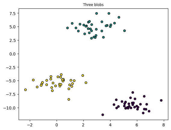
16.5.2. K-Means Clustering#
# https://towardsdatascience.com/machine-learning-algorithms-part-9-k-means-example-in-python-f2ad05ed5203
# https://blog.floydhub.com/introduction-to-k-means-clustering-in-python-with-scikit-learn/
from sklearn.datasets import make_blobs
plt.title("Three blobs", fontsize='small')
X1, Y1 = make_blobs(n_features=2, centers=3, random_state=10)
plt.scatter(X1[:, 0], X1[:, 1], marker='o', c=Y1,
            s=25, edgecolor='k')
Text(0.5, 1.0, 'Three blobs')
<matplotlib.collections.PathCollection at 0x714c4c373bc0>
16.5.3. Using scikit-learn to perform K-Means clustering#
from sklearn.cluster import KMeans

# Specify the number of clusters (3) and fit the data X
kmeans = KMeans(n_clusters=3, random_state=0).fit(X1)
# Get the cluster centroids

# Plotting the cluster centers and the data points on a 2D plane
plt.scatter(X1[:, 0], X1[:, 1], marker='o', c=Y1,
            s=25, edgecolor='k')

plt.scatter(kmeans.cluster_centers_[:, 0], kmeans.cluster_centers_[:, 1], c='red', marker='x')

plt.title('Data points and cluster centroids')
plt.show()
<matplotlib.collections.PathCollection at 0x714c4c081c10>
<matplotlib.collections.PathCollection at 0x714c4c1291f0>
Text(0.5, 1.0, 'Data points and cluster centroids')

16.5.3.1. Some links#
https://jakevdp.github.io/PythonDataScienceHandbook/05.07-support-vector-machines.html https://scikit-learn.org/stable/auto_examples/linear_model/plot_ransac.html http://www.cse.psu.edu/~rtc12/CSE486/lecture15.pdf https://towardsdatascience.com/accuracy-precision-recall-or-f1-331fb37c5cb9
16.5.4. Evaluating Algorithms#
from sklearn.datasets import load_breast_cancer
data = load_breast_cancer()
X = data.data
Y = data.target

from sklearn.metrics import accuracy_score
from sklearn.metrics import confusion_matrix
from sklearn.metrics import classification_report
from sklearn.model_selection import train_test_split
X_train, X_test, Y_train, Y_test = train_test_split(X, Y, test_size = 0.25, random_state = 0)
from sklearn.preprocessing import StandardScaler
sc = StandardScaler()
X_train = sc.fit_transform(X_train)
X_test = sc.transform(X_test)

from sklearn.linear_model import LogisticRegression
classifier = LogisticRegression(random_state = 0)
classifier.fit(X_train, Y_train)
Y_pred = classifier.predict(X_test)

accuracy = accuracy_score(Y_test, Y_pred)
accuracy
LogisticRegression(random_state=0)In a Jupyter environment, please rerun this cell to show the HTML representation or trust the notebook.
On GitHub, the HTML representation is unable to render, please try loading this page with nbviewer.org.
LogisticRegression(random_state=0)
0.958041958041958
cm = confusion_matrix(Y_test, Y_pred)
cm
# tn, fp, fn, tp = confusion_matrix(Y_test, Y_pred).ravel()
#TN, FP, FN, TP
#

- Sensitivity refers to a test's ability to designate an individual with disease as positive. A highly sensitive test means that there are few false negative results, and thus fewer cases of disease are missed.
- The specificity of a test is its ability to designate an individual who does not have a disease as negative.
- https://en.wikipedia.org/wiki/Confusion_matrix
  Cell In[26], line 7
    - Sensitivity refers to a test's ability to designate an individual with disease as positive. A highly sensitive test means that there are few false negative results, and thus fewer cases of disease are missed.
                                  ^
SyntaxError: unterminated string literal (detected at line 7)
tn, fp, fn, tp = confusion_matrix(Y_test, Y_pred).ravel()
tn
fp
fn
tp
# 380 b
# 20 m

TN = 380
TP = 0
TN, FP, FN, TP

https://stackoverflow.com/questions/56078203/why-scikit-learn-confusion-matrix-is-reversed

[[True Negative, False Positive]
[False Negative, True Positive]]
results = classification_report(Y_test, Y_pred)
print(results)
              precision    recall  f1-score   support

           0       0.94      0.94      0.94        53
           1       0.97      0.97      0.97        90

    accuracy                           0.96       143
   macro avg       0.96      0.96      0.96       143
weighted avg       0.96      0.96      0.96       143
# precision measures how accurate our positive predictions were
# precision = tp / (tp+fp)

# recall measures what fraction of the positives our model identified
# recall = tp / (tp+fn) -- same as sensitivity
16.5.4.1. Lots of Classifiers#
from sklearn.svm import SVC
classifier = SVC(kernel = 'rbf', random_state = 0)
classifier.fit(X_train, Y_train)
Y_pred = classifier.predict(X_test)
accuracy = accuracy_score(Y_test, Y_pred)
accuracy
cm = confusion_matrix(Y_test, Y_pred)
cm
SVC(random_state=0)In a Jupyter environment, please rerun this cell to show the HTML representation or trust the notebook.
On GitHub, the HTML representation is unable to render, please try loading this page with nbviewer.org.
SVC(random_state=0)
0.965034965034965
array([[50,  3],
       [ 2, 88]])
results = classification_report(Y_test, Y_pred)
print(results)
              precision    recall  f1-score   support

           0       0.96      0.94      0.95        53
           1       0.97      0.98      0.97        90

    accuracy                           0.97       143
   macro avg       0.96      0.96      0.96       143
weighted avg       0.96      0.97      0.96       143
from sklearn.naive_bayes import GaussianNB
classifier = GaussianNB()
classifier.fit(X_train, Y_train)
Y_pred = classifier.predict(X_test)
accuracy = accuracy_score(Y_test, Y_pred)
accuracy
cm = confusion_matrix(Y_test, Y_pred)
cm
GaussianNB()In a Jupyter environment, please rerun this cell to show the HTML representation or trust the notebook.
On GitHub, the HTML representation is unable to render, please try loading this page with nbviewer.org.
GaussianNB()
0.916083916083916
array([[47,  6],
       [ 6, 84]])
results = classification_report(Y_test, Y_pred)
print(results)
              precision    recall  f1-score   support

           0       0.89      0.89      0.89        53
           1       0.93      0.93      0.93        90

    accuracy                           0.92       143
   macro avg       0.91      0.91      0.91       143
weighted avg       0.92      0.92      0.92       143
from sklearn.tree import DecisionTreeClassifier
classifier = DecisionTreeClassifier(criterion = 'entropy', random_state = 0)
classifier.fit(X_train, Y_train)
Y_pred = classifier.predict(X_test)
accuracy = accuracy_score(Y_test, Y_pred)
accuracy
cm = confusion_matrix(Y_test, Y_pred)
cm
DecisionTreeClassifier(criterion='entropy', random_state=0)In a Jupyter environment, please rerun this cell to show the HTML representation or trust the notebook.
On GitHub, the HTML representation is unable to render, please try loading this page with nbviewer.org.
DecisionTreeClassifier(criterion='entropy', random_state=0)
0.958041958041958
array([[51,  2],
       [ 4, 86]])
results = classification_report(Y_test, Y_pred)
print(results)
              precision    recall  f1-score   support

           0       0.93      0.96      0.94        53
           1       0.98      0.96      0.97        90

    accuracy                           0.96       143
   macro avg       0.95      0.96      0.96       143
weighted avg       0.96      0.96      0.96       143
from sklearn.ensemble import RandomForestClassifier
classifier = RandomForestClassifier(n_estimators = 10, criterion = 'entropy', random_state = 0)
classifier.fit(X_train, Y_train)
Y_pred = classifier.predict(X_test)
accuracy = accuracy_score(Y_test, Y_pred)
accuracy
cm = confusion_matrix(Y_test, Y_pred)
cm

from sklearn.metrics import fbeta_score
output = fbeta_score(Y_test, Y_pred, average='macro', beta=0.5)
output
RandomForestClassifier(criterion='entropy', n_estimators=10, random_state=0)In a Jupyter environment, please rerun this cell to show the HTML representation or trust the notebook.
On GitHub, the HTML representation is unable to render, please try loading this page with nbviewer.org.
RandomForestClassifier(criterion='entropy', n_estimators=10, random_state=0)
0.972027972027972
array([[52,  1],
       [ 3, 87]])
np.float64(0.968271924154277)
16.5.4.1.1. Feature Importance#
for score, name in sorted(zip(classifier.feature_importances_, data.feature_names), reverse=True):
    print(round(score, 2), name)
0.14 mean concave points
0.14 worst perimeter
0.11 worst concave points
0.1 area error
0.08 worst area
0.06 mean concavity
0.05 radius error
0.05 mean area
0.04 worst radius
0.04 mean perimeter
0.03 mean texture
0.02 worst texture
0.02 worst fractal dimension
0.02 mean radius
0.01 perimeter error
0.01 worst concavity
0.01 concavity error
0.01 mean fractal dimension
0.01 mean smoothness
0.01 fractal dimension error
0.01 worst compactness
0.01 mean compactness
0.01 worst symmetry
0.01 concave points error
0.01 symmetry error
0.01 worst smoothness
0.0 compactness error
0.0 texture error
0.0 mean symmetry
0.0 smoothness error
results = classification_report(Y_test, Y_pred)
print(results)
X_train, X_test, Y_train, Y_test = train_test_split(X, Y, test_size = 0.2, random_state = 0)
sc = StandardScaler()
X_train = sc.fit_transform(X_train)
X_test = sc.transform(X_test)
classifier = LogisticRegression(random_state = 0)
classifier.fit(X_train, Y_train)
Y_pred = classifier.predict(X_test)

accuracy = accuracy_score(Y_test, Y_pred)
accuracy
cm = confusion_matrix(Y_test, Y_pred)
cm
LogisticRegression(random_state=0)In a Jupyter environment, please rerun this cell to show the HTML representation or trust the notebook.
On GitHub, the HTML representation is unable to render, please try loading this page with nbviewer.org.
LogisticRegression(random_state=0)
0.9649122807017544
array([[45,  2],
       [ 2, 65]])
from sklearn.metrics import classification_report
results = classification_report(Y_test, Y_pred)
print(results)
              precision    recall  f1-score   support

           0       0.96      0.96      0.96        47
           1       0.97      0.97      0.97        67

    accuracy                           0.96       114
   macro avg       0.96      0.96      0.96       114
weighted avg       0.96      0.96      0.96       114
from sklearn.metrics import roc_auc_score

roc_auc = roc_auc_score(Y_test, Y_pred)


from sklearn import metrics

fpr, tpr, thresholds = metrics.roc_curve(Y_test, Y_pred)
plt.figure()
lw = 2
plt.plot(
    fpr,
    tpr,
    color="darkorange",
    lw=lw,
    label="ROC curve (area = %0.2f)" % roc_auc,
)
plt.plot([0, 1], [0, 1], color="navy", lw=lw, linestyle="--")
plt.xlim([0.0, 1.0])
plt.ylim([0.0, 1.05])
plt.xlabel("False Positive Rate")
plt.ylabel("True Positive Rate")
plt.title("Receiver operating characteristic example")
plt.legend(loc="lower right")
plt.show()
<Figure size 640x480 with 0 Axes>
[<matplotlib.lines.Line2D at 0x714c483172f0>]
[<matplotlib.lines.Line2D at 0x714c4bca6870>]
(0.0, 1.0)
(0.0, 1.05)
Text(0.5, 0, 'False Positive Rate')
Text(0, 0.5, 'True Positive Rate')
Text(0.5, 1.0, 'Receiver operating characteristic example')
<matplotlib.legend.Legend at 0x714c4c081b20>

16.5.5. Imbalanced Data sets#
For imbalanced data sets, the AUC of precision/recall curve is more informative than the AUC for sensitivity/specificity curve.
https://www.kaggle.com/code/vedbharti/classification-precision-recall-vs-roc-plot
16.5.6. Stratify#
stratify
16.5.7. Vocabulary#
Supervised Learning
Unsupervised Learning
Classification
Prediction
Clustering
Cross-Validation
Dimensionality Reduction (curse of dimensionality)
Feature Selection
Accuracy
True Positive
True Negative
False Positive
False Negative
Confusion Matrix
Sensitivity
Specificity
Recall
Precision
F1-Score
Imbalanced Data
Area Under the Curve (Sensitivity/Specificity and Precision/Recall)
Underfitting
Overfitting – reduced via regularization (reduce degrees of freedom), early stopping (stop when validation error reaches minimum)
Bias – Error due to wrong assumptions, e.g., linear, when non linear; high-bias results in under fit training data
Variance – Excessive sensitivity to small variations in the training data; high results in over fitting.
Bias/Variance Trade-Off
Stratified Sampling