
Part 2
Contents
Part 2#
from IPython.core.interactiveshell import InteractiveShell
InteractiveShell.ast_node_interactivity = "all"
PCA#
import numpy as np
from scipy import signal
import matplotlib.pyplot as plt
%matplotlib inline
np.random.seed = 1
N = 1000
fs = 500
w = np.arange(1,N+1) * 2 * np.pi/fs
t = np.arange(1,N+1)/fs
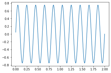
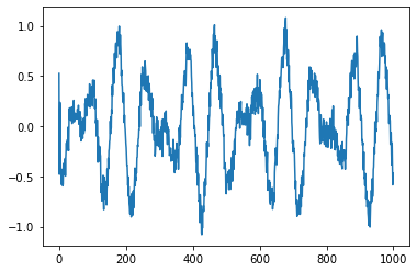
x = 0.75 * np.sin(w*5)
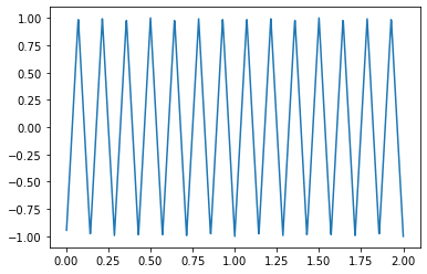
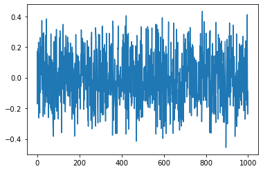
y = signal.sawtooth(w*7, 0.5)
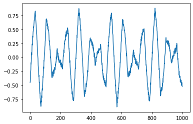
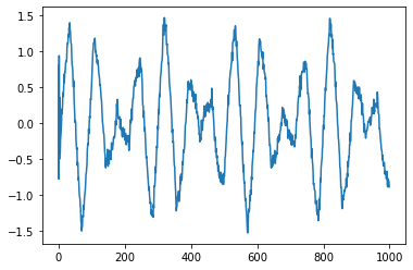
d1 = 0.5*y + 0.5*x + 0.1*np.random.rand(1,N)
d2 = 0.2*y + 0.75*x + 0.15*np.random.rand(1,N)
d3 = 0.7*y + 0.25*x + 0.1*np.random.rand(1,N)
d4 = -0.5*y + 0.4*x + 0.2*np.random.rand(1,N)
d5 = 0.6*np.random.rand(1,N)
d1 = d1 - d1.mean()
d2 = d2 - d2.mean()
d3 = d3 - d3.mean()
d4 = d4 - d4.mean()
d5 = d5 - d5.mean()
plt.plot(d1.transpose())
[<matplotlib.lines.Line2D at 0x7f0932433940>]
plt.plot(t, x)
[<matplotlib.lines.Line2D at 0x7f0931ba58e0>]
plt.plot(t, y)
[<matplotlib.lines.Line2D at 0x7f0931b22850>]
import numpy as np
X = np.array([d1[0], d2[0], d3[0], d4[0], d5[0]])
X
array([[-0.45292143, -0.44323002, -0.38876664, ..., -0.46883499,
        -0.51798614, -0.52302918],
       [-0.15001728, -0.12268033, -0.0644054 , ..., -0.22812214,
        -0.17648028, -0.23092364],
       [-0.64061745, -0.63109802, -0.5667706 , ..., -0.60187111,
        -0.64249032, -0.66368368],
       [ 0.5465051 ,  0.4655634 ,  0.41198267, ...,  0.38446487,
         0.42051796,  0.44459525],
       [ 0.2429415 ,  0.00965245,  0.00330278, ...,  0.17670271,
        -0.20930871,  0.13536191]])
X.shape
(5, 1000)
U,S,V = np.linalg.svd(X)
S
array([20.8807396 , 14.19645247, 5.38766041, 1.49581382, 0.97589064])
eigen = S**2
eigen
array([436.00528626, 201.53926275,  29.02688473,   2.23745899,
         0.95236254])
eigen
array([436.00528626, 201.53926275,  29.02688473,   2.23745899,
         0.95236254])
for i in range(5):
    V[:,i] = V[:,i] * np.sqrt(eigen[i])
eigen = eigen/N
eigen = eigen/sum(eigen)
eigen
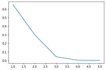
array([0.65098613, 0.3009121 , 0.04333915, 0.00334068, 0.00142194])
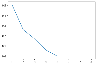
Scree plot#
Gives the measure of the associated principal component’s importance with regards to how much of the total information it represents.
plt.plot(range(1,6), eigen)
[<matplotlib.lines.Line2D at 0x7f0931a97c70>]
plt.plot(V[:,0])
plt.show()
[<matplotlib.lines.Line2D at 0x7f0931263310>]
plt.plot(V[:,1])
plt.show()
[<matplotlib.lines.Line2D at 0x7f0931244ac0>]
plt.plot(V[:,2])
plt.show()
[<matplotlib.lines.Line2D at 0x7f09311ab4c0>]
PCA on Iris Data#
import matplotlib.pyplot as plt
from mpl_toolkits.mplot3d import Axes3D
from sklearn import datasets
from sklearn.decomposition import PCA
# import some data to play with
iris = datasets.load_iris()
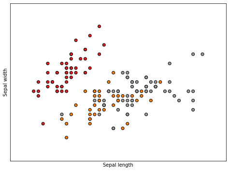
X = iris.data[:, :2] # we only take the first two features.
y = iris.target
x_min, x_max = X[:, 0].min() - .5, X[:, 0].max() + .5
y_min, y_max = X[:, 1].min() - .5, X[:, 1].max() + .5
plt.figure(2, figsize=(8, 6))
plt.clf()
# Plot the training points
plt.scatter(X[:, 0], X[:, 1], c=y, cmap=plt.cm.Set1,
edgecolor='k')
plt.xlabel('Sepal length')
plt.ylabel('Sepal width')
plt.xlim(x_min, x_max)
plt.ylim(y_min, y_max)
plt.xticks(())
plt.yticks(())
# To getter a better understanding of interaction of the dimensions
# plot the first three PCA dimensions
fig = plt.figure(1, figsize=(8, 6))
ax = Axes3D(fig, elev=-150, azim=110)
X_reduced = PCA(n_components=3).fit_transform(iris.data)
ax.scatter(X_reduced[:, 0], X_reduced[:, 1], X_reduced[:, 2], c=y,
cmap=plt.cm.Set1, edgecolor='k', s=40)
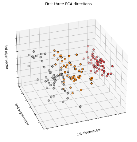
ax.set_title("First three PCA directions")
ax.set_xlabel("1st eigenvector")
ax.w_xaxis.set_ticklabels([])
ax.set_ylabel("2nd eigenvector")
ax.w_yaxis.set_ticklabels([])
ax.set_zlabel("3rd eigenvector")
ax.w_zaxis.set_ticklabels([])
plt.show()
<Figure size 576x432 with 0 Axes>
<matplotlib.collections.PathCollection at 0x7f092eead7f0>
Text(0.5, 0, 'Sepal length')
Text(0, 0.5, 'Sepal width')
(3.8, 8.4)
(1.5, 4.9)
([], [])
([], [])
/tmp/ipykernel_280/1367415577.py:31: MatplotlibDeprecationWarning: Axes3D(fig) adding itself to the figure is deprecated since 3.4. Pass the keyword argument auto_add_to_figure=False and use fig.add_axes(ax) to suppress this warning. The default value of auto_add_to_figure will change to False in mpl3.5 and True values will no longer work in 3.6.  This is consistent with other Axes classes.
  ax = Axes3D(fig, elev=-150, azim=110)
<mpl_toolkits.mplot3d.art3d.Path3DCollection at 0x7f092ee81f70>
Text(0.5, 0.92, 'First three PCA directions')
Text(0.5, 0, '1st eigenvector')
[Text(-4.0, 0, ''),
 Text(-3.0, 0, ''),
 Text(-2.0, 0, ''),
 Text(-1.0, 0, ''),
 Text(0.0, 0, ''),
 Text(1.0, 0, ''),
 Text(2.0, 0, ''),
 Text(3.0, 0, ''),
 Text(4.0, 0, ''),
 Text(5.0, 0, '')]
Text(0.5, 0.5, '2nd eigenvector')
[Text(-1.5, 0, ''),
 Text(-1.0, 0, ''),
 Text(-0.5, 0, ''),
 Text(0.0, 0, ''),
 Text(0.5, 0, ''),
 Text(1.0, 0, ''),
 Text(1.5, 0, ''),
 Text(2.0, 0, '')]
Text(0.5, 0, '3rd eigenvector')
[Text(-0.8, 0, ''),
 Text(-0.6000000000000001, 0, ''),
 Text(-0.4, 0, ''),
 Text(-0.19999999999999996, 0, ''),
 Text(0.0, 0, ''),
 Text(0.19999999999999996, 0, ''),
 Text(0.40000000000000013, 0, ''),
 Text(0.6000000000000001, 0, ''),
 Text(0.8, 0, ''),
 Text(1.0, 0, '')]
iris = datasets.load_iris()
X = iris.data[:50,:]
X2 = X +0.05*np.random.rand(50,4)
X_combined = np.zeros((50,8))
X_combined[:,0:4] = X
X_combined[:,4:] = X2
X_combined
array([[5.1       , 3.5       , 1.4       , 0.2       , 5.14620352,
        3.50263533, 1.43276678, 0.23023365],
       [4.9       , 3.        , 1.4       , 0.2       , 4.92153394,
        3.0451091 , 1.41850911, 0.24347364],
       [4.7       , 3.2       , 1.3       , 0.2       , 4.72220228,
        3.21979427, 1.32109586, 0.24705178],
       [4.6       , 3.1       , 1.5       , 0.2       , 4.63346086,
        3.12972135, 1.51061918, 0.20370002],
       [5.        , 3.6       , 1.4       , 0.2       , 5.01541827,
        3.61694033, 1.44194588, 0.20988829],
       [5.4       , 3.9       , 1.7       , 0.4       , 5.43205806,
        3.91326706, 1.73567529, 0.42082037],
       [4.6       , 3.4       , 1.4       , 0.3       , 4.60339603,
        3.44035131, 1.40173254, 0.3399996 ],
       [5.        , 3.4       , 1.5       , 0.2       , 5.02891321,
        3.44845173, 1.53810547, 0.21885036],
       [4.4       , 2.9       , 1.4       , 0.2       , 4.43113992,
        2.94966446, 1.42355072, 0.23062666],
       [4.9       , 3.1       , 1.5       , 0.1       , 4.90580716,
        3.1449495 , 1.53916881, 0.1184625 ],
       [5.4       , 3.7       , 1.5       , 0.2       , 5.41855454,
        3.71625948, 1.54150824, 0.23352735],
       [4.8       , 3.4       , 1.6       , 0.2       , 4.84515745,
        3.40814182, 1.62082618, 0.20655399],
       [4.8       , 3.        , 1.4       , 0.1       , 4.80301068,
        3.02898664, 1.42829241, 0.12314783],
       [4.3       , 3.        , 1.1       , 0.1       , 4.32882268,
        3.018308  , 1.11534999, 0.14968448],
       [5.8       , 4.        , 1.2       , 0.2       , 5.81269442,
        4.04671768, 1.20881284, 0.20821636],
       [5.7       , 4.4       , 1.5       , 0.4       , 5.70668532,
        4.44422102, 1.51243261, 0.42580091],
       [5.4       , 3.9       , 1.3       , 0.4       , 5.41672088,
        3.927448  , 1.30831317, 0.41194794],
       [5.1       , 3.5       , 1.4       , 0.3       , 5.1476249 ,
        3.5469883 , 1.44524539, 0.31463397],
       [5.7       , 3.8       , 1.7       , 0.3       , 5.73304258,
        3.82078294, 1.73738306, 0.31931736],
       [5.1       , 3.8       , 1.5       , 0.3       , 5.1090606 ,
        3.82322265, 1.52229342, 0.32932551],
       [5.4       , 3.4       , 1.7       , 0.2       , 5.42229364,
        3.4133437 , 1.71591301, 0.23293349],
       [5.1       , 3.7       , 1.5       , 0.4       , 5.14615383,
        3.73180139, 1.53559472, 0.42487537],
       [4.6       , 3.6       , 1.        , 0.2       , 4.61410762,
        3.60154486, 1.04993929, 0.22164826],
       [5.1       , 3.3       , 1.7       , 0.5       , 5.10819008,
        3.34828889, 1.74573479, 0.51251163],
       [4.8       , 3.4       , 1.9       , 0.2       , 4.8089392 ,
        3.41718691, 1.9307314 , 0.23862259],
       [5.        , 3.        , 1.6       , 0.2       , 5.02443907,
        3.03084477, 1.62101889, 0.24855046],
       [5.        , 3.4       , 1.6       , 0.4       , 5.0011145 ,
        3.44193054, 1.64991472, 0.4498733 ],
       [5.2       , 3.5       , 1.5       , 0.2       , 5.22300348,
        3.50630915, 1.52981806, 0.20104765],
       [5.2       , 3.4       , 1.4       , 0.2       , 5.22774343,
        3.42522333, 1.44021092, 0.23772789],
       [4.7       , 3.2       , 1.6       , 0.2       , 4.70407051,
        3.24326544, 1.6333866 , 0.2470641 ],
       [4.8       , 3.1       , 1.6       , 0.2       , 4.81290199,
        3.11631918, 1.60670437, 0.24586371],
       [5.4       , 3.4       , 1.5       , 0.4       , 5.44807388,
        3.40449458, 1.53674072, 0.44809678],
       [5.2       , 4.1       , 1.5       , 0.1       , 5.21205465,
        4.11444309, 1.51019967, 0.14366238],
       [5.5       , 4.2       , 1.4       , 0.2       , 5.50155761,
        4.23106238, 1.4170138 , 0.2431729 ],
       [4.9       , 3.1       , 1.5       , 0.2       , 4.9346635 ,
        3.13973697, 1.51623182, 0.24231851],
       [5.        , 3.2       , 1.2       , 0.2       , 5.00727284,
        3.21307191, 1.20723018, 0.24425854],
       [5.5       , 3.5       , 1.3       , 0.2       , 5.51064691,
        3.50395621, 1.3309535 , 0.2424406 ],
       [4.9       , 3.6       , 1.4       , 0.1       , 4.92091772,
        3.64045614, 1.43707993, 0.10650626],
       [4.4       , 3.        , 1.3       , 0.2       , 4.42933367,
        3.01377284, 1.32112949, 0.22707754],
       [5.1       , 3.4       , 1.5       , 0.2       , 5.10443227,
        3.41556643, 1.50106239, 0.23353087],
       [5.        , 3.5       , 1.3       , 0.3       , 5.01199456,
        3.53929502, 1.32399731, 0.30309266],
       [4.5       , 2.3       , 1.3       , 0.3       , 4.53734536,
        2.30437783, 1.32306741, 0.34096505],
       [4.4       , 3.2       , 1.3       , 0.2       , 4.43596034,
        3.21712868, 1.32155137, 0.21776906],
       [5.        , 3.5       , 1.6       , 0.6       , 5.01826435,
        3.50762634, 1.63515978, 0.62161351],
       [5.1       , 3.8       , 1.9       , 0.4       , 5.10367042,
        3.84136483, 1.9119218 , 0.40517719],
       [4.8       , 3.        , 1.4       , 0.3       , 4.83154727,
        3.00713961, 1.41337727, 0.33252103],
       [5.1       , 3.8       , 1.6       , 0.2       , 5.14628465,
        3.80676924, 1.62429618, 0.20089096],
       [4.6       , 3.2       , 1.4       , 0.2       , 4.62538179,
        3.23273068, 1.4459905 , 0.22853028],
       [5.3       , 3.7       , 1.5       , 0.2       , 5.34538422,
        3.70566099, 1.52285264, 0.22666238],
       [5.        , 3.3       , 1.4       , 0.2       , 5.03579419,
        3.32282104, 1.431169  , 0.22751033]])
X_combined.mean(axis=0)
array([5.006     , 3.428     , 1.462     , 0.246     , 5.0283009 ,
       3.45258988, 1.48787237, 0.27363556])
from sklearn import preprocessing
X_scaled = preprocessing.scale(X_combined)
X_scaled
array([[ 2.69381893e-01,  1.91869743e-01, -3.60635820e-01,
        -4.40923824e-01,  3.38934023e-01,  1.33073309e-01,
        -3.17786950e-01, -4.19552910e-01],
       [-3.03771071e-01, -1.14055903e+00, -3.60635820e-01,
        -4.40923824e-01, -3.06922369e-01, -1.08351128e+00,
        -4.00009111e-01, -2.91566032e-01],
       [-8.76924035e-01, -6.07587521e-01, -9.42306497e-01,
        -4.40923824e-01, -8.79939993e-01, -6.19014894e-01,
        -9.61778975e-01, -2.56977237e-01],
       [-1.16350052e+00, -8.74073275e-01,  2.21034857e-01,
        -4.40923824e-01, -1.13504445e+00, -8.58523183e-01,
         1.31177940e-01, -6.76045357e-01],
       [-1.71945889e-02,  4.58355498e-01, -3.60635820e-01,
        -4.40923824e-01, -3.70336066e-02,  4.37015874e-01,
        -2.64852262e-01, -6.16225232e-01],
       [ 1.12911134e+00,  1.25781276e+00,  1.38437621e+00,
         1.47613628e+00,  1.16067845e+00,  1.22496313e+00,
         1.42904796e+00,  1.42279038e+00],
       [-1.16350052e+00, -7.46160113e-02, -3.60635820e-01,
         5.17606228e-01, -1.22147165e+00, -3.25429500e-02,
        -4.96757445e-01,  6.41520827e-01],
       [-1.71945889e-02, -7.46160113e-02,  2.21034857e-01,
        -4.40923824e-01,  1.76020064e-03, -1.10035411e-02,
         2.89687905e-01, -5.29591648e-01],
       [-1.73665348e+00, -1.40704478e+00, -3.60635820e-01,
        -4.40923824e-01, -1.71665532e+00, -1.33730326e+00,
        -3.70934798e-01, -4.15753807e-01],
       [-3.03771071e-01, -8.74073275e-01,  2.21034857e-01,
        -1.39945388e+00, -3.52132054e-01, -8.18030781e-01,
         2.95820042e-01, -1.50001031e+00],
       [ 1.12911134e+00,  7.24841253e-01,  2.21034857e-01,
        -4.40923824e-01,  1.12185996e+00,  7.01110342e-01,
         3.09311239e-01, -3.87713739e-01],
       [-5.90347553e-01, -7.46160113e-02,  8.02705535e-01,
        -4.40923824e-01, -5.26481452e-01, -1.18189561e-01,
         7.66727750e-01, -6.48456923e-01],
       [-5.90347553e-01, -1.14055903e+00, -3.60635820e-01,
        -1.39945388e+00, -6.47640519e-01, -1.12638169e+00,
        -3.43590042e-01, -1.45471866e+00],
       [-2.02322996e+00, -1.14055903e+00, -2.10564785e+00,
        -1.39945388e+00, -2.01078613e+00, -1.15477672e+00,
        -2.14828922e+00, -1.19819705e+00],
       [ 2.27541727e+00,  1.52429852e+00, -1.52397717e+00,
        -4.40923824e-01,  2.25489169e+00,  1.57981483e+00,
        -1.60930087e+00, -6.32387331e-01],
       [ 1.98884078e+00,  2.59024154e+00,  2.21034857e-01,
         1.47613628e+00,  1.95014792e+00,  2.63679564e+00,
         1.41635768e-01,  1.47093577e+00],
       [ 1.12911134e+00,  1.25781276e+00, -9.42306497e-01,
         1.47613628e+00,  1.11658877e+00,  1.26267092e+00,
        -1.03549507e+00,  1.33702332e+00],
       [ 2.69381893e-01,  1.91869743e-01, -3.60635820e-01,
         5.17606228e-01,  3.43020045e-01,  2.51009997e-01,
        -2.45824362e-01,  3.96319062e-01],
       [ 1.98884078e+00,  9.91327007e-01,  1.38437621e+00,
         5.17606228e-01,  2.02591697e+00,  9.79043316e-01,
         1.43889648e+00,  4.41591996e-01],
       [ 2.69381893e-01,  9.91327007e-01,  2.21034857e-01,
         5.17606228e-01,  2.32159477e-01,  9.85530644e-01,
         1.98501814e-01,  5.38337710e-01],
       [ 1.12911134e+00, -7.46160113e-02,  1.38437621e+00,
        -4.40923824e-01,  1.13260873e+00, -1.04357508e-01,
         1.31508139e+00, -3.93454429e-01],
       [ 2.69381893e-01,  7.24841253e-01,  2.21034857e-01,
         1.47613628e+00,  3.38791170e-01,  7.42437044e-01,
         2.75208723e-01,  1.46198881e+00],
       [-1.16350052e+00,  4.58355498e-01, -2.68731853e+00,
        -4.40923824e-01, -1.19067909e+00,  3.96078567e-01,
        -2.52550446e+00, -5.02545242e-01],
       [ 2.69381893e-01, -3.41101766e-01,  1.38437621e+00,
         2.43466633e+00,  2.29656978e-01, -2.77341433e-01,
         1.48705985e+00,  2.30914168e+00],
       [-5.90347553e-01, -7.46160113e-02,  2.54771757e+00,
        -4.40923824e-01, -6.30597844e-01, -9.41382267e-02,
         2.55391179e+00, -3.38459562e-01],
       [-1.71945889e-02, -1.14055903e+00,  8.02705535e-01,
        -4.40923824e-01, -1.11015734e-02, -1.12144083e+00,
         7.67839075e-01, -2.42489895e-01],
       [-1.71945889e-02, -7.46160113e-02,  8.02705535e-01,
         1.47613628e+00, -7.81525851e-02, -2.83437076e-02,
         9.34477665e-01,  1.70363612e+00],
       [ 5.55958375e-01,  1.91869743e-01,  2.21034857e-01,
        -4.40923824e-01,  5.59710428e-01,  1.42842171e-01,
         2.41895438e-01, -7.01685026e-01],
       [ 5.55958375e-01, -7.46160113e-02, -3.60635820e-01,
        -4.40923824e-01,  5.73336332e-01, -7.27689870e-02,
        -2.74857512e-01, -3.47108414e-01],
       [-8.76924035e-01, -6.07587521e-01,  8.02705535e-01,
        -4.40923824e-01, -9.32063271e-01, -5.56603905e-01,
         8.39162084e-01, -2.56858154e-01],
       [-5.90347553e-01, -8.74073275e-01,  8.02705535e-01,
        -4.40923824e-01, -6.19206044e-01, -8.94160212e-01,
         6.85289052e-01, -2.68461944e-01],
       [ 1.12911134e+00, -7.46160113e-02,  2.21034857e-01,
         1.47613628e+00,  1.20671905e+00, -1.27887742e-01,
         2.81817581e-01,  1.68646309e+00],
       [ 5.55958375e-01,  1.79078427e+00,  2.21034857e-01,
        -1.39945388e+00,  5.28235882e-01,  1.75990001e+00,
         1.28758680e-01, -1.25641077e+00],
       [ 1.41568782e+00,  2.05727003e+00, -3.60635820e-01,
        -4.40923824e-01,  1.36046843e+00,  2.06999638e+00,
        -4.08632351e-01, -2.94473137e-01],
       [-3.03771071e-01, -8.74073275e-01,  2.21034857e-01,
        -4.40923824e-01, -2.69178890e-01, -8.31891161e-01,
         1.63545364e-01, -3.02732314e-01],
       [-1.71945889e-02, -6.07587521e-01, -1.52397717e+00,
        -4.40923824e-01, -6.04492346e-02, -6.36889979e-01,
        -1.61842787e+00, -2.83978653e-01],
       [ 1.41568782e+00,  1.91869743e-01, -9.42306497e-01,
        -4.40923824e-01,  1.38659738e+00,  1.36585575e-01,
        -9.04931168e-01, -3.01552051e-01],
       [-3.03771071e-01,  4.58355498e-01, -3.60635820e-01,
        -1.39945388e+00, -3.08693804e-01,  4.99545568e-01,
        -2.92913549e-01, -1.61558758e+00],
       [-1.73665348e+00, -1.14055903e+00, -9.42306497e-01,
        -4.40923824e-01, -1.72184774e+00, -1.16683594e+00,
        -9.61584986e-01, -4.50062042e-01],
       [ 2.69381893e-01, -7.46160113e-02,  2.21034857e-01,
        -4.40923824e-01,  2.18854419e-01, -9.84471608e-02,
         7.60651948e-02, -3.87679696e-01],
       [-1.71945889e-02,  1.91869743e-01, -9.42306497e-01,
         5.17606228e-01, -4.68757424e-02,  2.30553212e-01,
        -9.45046655e-01,  2.84752780e-01],
       [-1.45007700e+00, -3.00595931e+00, -9.42306497e-01,
         5.17606228e-01, -1.41134715e+00, -3.05315189e+00,
        -9.50409266e-01,  6.50853568e-01],
       [-1.73665348e+00, -6.07587521e-01, -9.42306497e-01,
        -4.40923824e-01, -1.70279809e+00, -6.26102834e-01,
        -9.59152082e-01, -5.40044287e-01],
       [-1.71945889e-02,  1.91869743e-01,  8.02705535e-01,
         3.39319638e+00, -2.88520024e-02,  1.46344631e-01,
         8.49387791e-01,  3.36379607e+00],
       [ 2.69381893e-01,  9.91327007e-01,  2.54771757e+00,
         1.47613628e+00,  2.16664344e-01,  1.03377158e+00,
         2.44543920e+00,  1.27157259e+00],
       [-5.90347553e-01, -1.14055903e+00, -3.60635820e-01,
         5.17606228e-01, -5.65606554e-01, -1.18447401e+00,
        -4.29603771e-01,  5.69227824e-01],
       [ 2.69381893e-01,  9.91327007e-01,  8.02705535e-01,
        -4.40923824e-01,  3.39167242e-01,  9.41780221e-01,
         7.86738786e-01, -7.03199655e-01],
       [-1.16350052e+00, -6.07587521e-01, -3.60635820e-01,
        -4.40923824e-01, -1.15826931e+00, -5.84616346e-01,
        -2.41527417e-01, -4.36018821e-01],
       [ 8.42534857e-01,  7.24841253e-01,  2.21034857e-01,
        -4.40923824e-01,  9.11517647e-01,  6.72928453e-01,
         2.01726757e-01, -4.54075292e-01],
       [-1.71945889e-02, -3.41101766e-01, -3.60635820e-01,
        -4.40923824e-01,  2.15409249e-02, -3.45061680e-01,
        -3.27001123e-01, -4.45878387e-01]])
X_scaled.mean(axis=0)
array([ 1.87003191e-15, -2.20823360e-15, -1.17128529e-15,  9.17044218e-16,
       -2.84931800e-15,  2.40918396e-15,  1.34559031e-15,  1.44328993e-17])
U,S,V = np.linalg.svd(X_scaled)
S
array([14.28769107, 10.15143438,  8.16514049,  5.04781531,  0.67298288,
        0.36423881,  0.22510887,  0.15509746])
eigen = S**2
eigen
array([2.04138116e+02, 1.03051620e+02, 6.66695193e+01, 2.54804394e+01,
       4.52905952e-01, 1.32669908e-01, 5.06740018e-02, 2.40552214e-02])
eigen = eigen/50
eigen = eigen/sum(eigen)
eigen = np.round(eigen*100)/100
print(eigen)
[0.51 0.26 0.17 0.06 0. 0. 0. 0. ]
sum([0.51, 0.26, 0.17, 0.06])
1.0
plt.plot(range(1, 9), eigen)
[<matplotlib.lines.Line2D at 0x7f092d5aea30>]
X_reduced = PCA(n_components=3).fit_transform(X_scaled)
# https://towardsdatascience.com/machine-learning-algorithms-part-9-k-means-example-in-python-f2ad05ed5203
# https://blog.floydhub.com/introduction-to-k-means-clustering-in-python-with-scikit-learn/
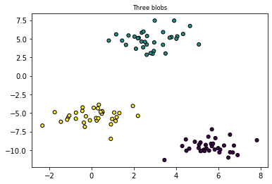
from sklearn.datasets import make_blobs
plt.title("Three blobs", fontsize='small')
X1, Y1 = make_blobs(n_features=2, centers=3, random_state=10)
plt.scatter(X1[:, 0], X1[:, 1], marker='o', c=Y1,
s=25, edgecolor='k')
Text(0.5, 1.0, 'Three blobs')
<matplotlib.collections.PathCollection at 0x7f092d5177c0>
# Using scikit-learn to perform K-Means clustering
from sklearn.cluster import KMeans
# Specify the number of clusters (3) and fit the data X
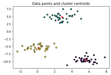
kmeans = KMeans(n_clusters=3, random_state=0).fit(X1)
# Get the cluster centroids
# Plotting the cluster centers and the data points on a 2D plane
plt.scatter(X1[:, 0], X1[:, 1], marker='o', c=Y1,
s=25, edgecolor='k')
plt.scatter(kmeans.cluster_centers_[:, 0], kmeans.cluster_centers_[:, 1], c='red', marker='x')
plt.title('Data points and cluster centroids')
plt.show()
<matplotlib.collections.PathCollection at 0x7f092c799c70>
<matplotlib.collections.PathCollection at 0x7f092d547eb0>
Text(0.5, 1.0, 'Data points and cluster centroids')
# https://jakevdp.github.io/PythonDataScienceHandbook/05.07-support-vector-machines.html
# https://scikit-learn.org/stable/auto_examples/linear_model/plot_ransac.html
# http://www.cse.psu.edu/~rtc12/CSE486/lecture15.pdf
# https://towardsdatascience.com/accuracy-precision-recall-or-f1-331fb37c5cb9
Evaluating Algorithms#
from sklearn.datasets import load_breast_cancer
data = load_breast_cancer()
X = data.data
Y = data.target

from sklearn.metrics import accuracy_score
from sklearn.metrics import confusion_matrix
from sklearn.metrics import classification_report
print(data.DESCR)
data.target_names
.. _breast_cancer_dataset:

Breast cancer wisconsin (diagnostic) dataset
--------------------------------------------

**Data Set Characteristics:**

    :Number of Instances: 569

    :Number of Attributes: 30 numeric, predictive attributes and the class

    :Attribute Information:
        - radius (mean of distances from center to points on the perimeter)
        - texture (standard deviation of gray-scale values)
        - perimeter
        - area
        - smoothness (local variation in radius lengths)
        - compactness (perimeter^2 / area - 1.0)
        - concavity (severity of concave portions of the contour)
        - concave points (number of concave portions of the contour)
        - symmetry
        - fractal dimension ("coastline approximation" - 1)

        The mean, standard error, and "worst" or largest (mean of the three
        worst/largest values) of these features were computed for each image,
        resulting in 30 features.  For instance, field 0 is Mean Radius, field
        10 is Radius SE, field 20 is Worst Radius.

        - class:
                - WDBC-Malignant
                - WDBC-Benign

    :Summary Statistics:

    ===================================== ====== ======
                                           Min    Max
    ===================================== ====== ======
    radius (mean):                        6.981  28.11
    texture (mean):                       9.71   39.28
    perimeter (mean):                     43.79  188.5
    area (mean):                          143.5  2501.0
    smoothness (mean):                    0.053  0.163
    compactness (mean):                   0.019  0.345
    concavity (mean):                     0.0    0.427
    concave points (mean):                0.0    0.201
    symmetry (mean):                      0.106  0.304
    fractal dimension (mean):             0.05   0.097
    radius (standard error):              0.112  2.873
    texture (standard error):             0.36   4.885
    perimeter (standard error):           0.757  21.98
    area (standard error):                6.802  542.2
    smoothness (standard error):          0.002  0.031
    compactness (standard error):         0.002  0.135
    concavity (standard error):           0.0    0.396
    concave points (standard error):      0.0    0.053
    symmetry (standard error):            0.008  0.079
    fractal dimension (standard error):   0.001  0.03
    radius (worst):                       7.93   36.04
    texture (worst):                      12.02  49.54
    perimeter (worst):                    50.41  251.2
    area (worst):                         185.2  4254.0
    smoothness (worst):                   0.071  0.223
    compactness (worst):                  0.027  1.058
    concavity (worst):                    0.0    1.252
    concave points (worst):               0.0    0.291
    symmetry (worst):                     0.156  0.664
    fractal dimension (worst):            0.055  0.208
    ===================================== ====== ======

    :Missing Attribute Values: None

    :Class Distribution: 212 - Malignant, 357 - Benign

    :Creator:  Dr. William H. Wolberg, W. Nick Street, Olvi L. Mangasarian

    :Donor: Nick Street

    :Date: November, 1995

This is a copy of UCI ML Breast Cancer Wisconsin (Diagnostic) datasets.
https://goo.gl/U2Uwz2

Features are computed from a digitized image of a fine needle
aspirate (FNA) of a breast mass.  They describe
characteristics of the cell nuclei present in the image.

Separating plane described above was obtained using
Multisurface Method-Tree (MSM-T) [K. P. Bennett, "Decision Tree
Construction Via Linear Programming." Proceedings of the 4th
Midwest Artificial Intelligence and Cognitive Science Society,
pp. 97-101, 1992], a classification method which uses linear
programming to construct a decision tree.  Relevant features
were selected using an exhaustive search in the space of 1-4
features and 1-3 separating planes.

The actual linear program used to obtain the separating plane
in the 3-dimensional space is that described in:
[K. P. Bennett and O. L. Mangasarian: "Robust Linear
Programming Discrimination of Two Linearly Inseparable Sets",
Optimization Methods and Software 1, 1992, 23-34].

This database is also available through the UW CS ftp server:

ftp ftp.cs.wisc.edu
cd math-prog/cpo-dataset/machine-learn/WDBC/

.. topic:: References

   - W.N. Street, W.H. Wolberg and O.L. Mangasarian. Nuclear feature extraction
     for breast tumor diagnosis. IS&T/SPIE 1993 International Symposium on
     Electronic Imaging: Science and Technology, volume 1905, pages 861-870,
     San Jose, CA, 1993.
   - O.L. Mangasarian, W.N. Street and W.H. Wolberg. Breast cancer diagnosis and
     prognosis via linear programming. Operations Research, 43(4), pages 570-577,
     July-August 1995.
   - W.H. Wolberg, W.N. Street, and O.L. Mangasarian. Machine learning techniques
     to diagnose breast cancer from fine-needle aspirates. Cancer Letters 77 (1994)
     163-171.
array(['malignant', 'benign'], dtype='<U9')
data.target
array([0, 0, 0, 0, 0, 0, 0, 0, 0, 0, 0, 0, 0, 0, 0, 0, 0, 0, 0, 1, 1, 1,
       0, 0, 0, 0, 0, 0, 0, 0, 0, 0, 0, 0, 0, 0, 0, 1, 0, 0, 0, 0, 0, 0,
       0, 0, 1, 0, 1, 1, 1, 1, 1, 0, 0, 1, 0, 0, 1, 1, 1, 1, 0, 1, 0, 0,
       1, 1, 1, 1, 0, 1, 0, 0, 1, 0, 1, 0, 0, 1, 1, 1, 0, 0, 1, 0, 0, 0,
       1, 1, 1, 0, 1, 1, 0, 0, 1, 1, 1, 0, 0, 1, 1, 1, 1, 0, 1, 1, 0, 1,
       1, 1, 1, 1, 1, 1, 1, 0, 0, 0, 1, 0, 0, 1, 1, 1, 0, 0, 1, 0, 1, 0,
       0, 1, 0, 0, 1, 1, 0, 1, 1, 0, 1, 1, 1, 1, 0, 1, 1, 1, 1, 1, 1, 1,
       1, 1, 0, 1, 1, 1, 1, 0, 0, 1, 0, 1, 1, 0, 0, 1, 1, 0, 0, 1, 1, 1,
       1, 0, 1, 1, 0, 0, 0, 1, 0, 1, 0, 1, 1, 1, 0, 1, 1, 0, 0, 1, 0, 0,
       0, 0, 1, 0, 0, 0, 1, 0, 1, 0, 1, 1, 0, 1, 0, 0, 0, 0, 1, 1, 0, 0,
       1, 1, 1, 0, 1, 1, 1, 1, 1, 0, 0, 1, 1, 0, 1, 1, 0, 0, 1, 0, 1, 1,
       1, 1, 0, 1, 1, 1, 1, 1, 0, 1, 0, 0, 0, 0, 0, 0, 0, 0, 0, 0, 0, 0,
       0, 0, 1, 1, 1, 1, 1, 1, 0, 1, 0, 1, 1, 0, 1, 1, 0, 1, 0, 0, 1, 1,
       1, 1, 1, 1, 1, 1, 1, 1, 1, 1, 1, 0, 1, 1, 0, 1, 0, 1, 1, 1, 1, 1,
       1, 1, 1, 1, 1, 1, 1, 1, 1, 0, 1, 1, 1, 0, 1, 0, 1, 1, 1, 1, 0, 0,
       0, 1, 1, 1, 1, 0, 1, 0, 1, 0, 1, 1, 1, 0, 1, 1, 1, 1, 1, 1, 1, 0,
       0, 0, 1, 1, 1, 1, 1, 1, 1, 1, 1, 1, 1, 0, 0, 1, 0, 0, 0, 1, 0, 0,
       1, 1, 1, 1, 1, 0, 1, 1, 1, 1, 1, 0, 1, 1, 1, 0, 1, 1, 0, 0, 1, 1,
       1, 1, 1, 1, 0, 1, 1, 1, 1, 1, 1, 1, 0, 1, 1, 1, 1, 1, 0, 1, 1, 0,
       1, 1, 1, 1, 1, 1, 1, 1, 1, 1, 1, 1, 0, 1, 0, 0, 1, 0, 1, 1, 1, 1,
       1, 0, 1, 1, 0, 1, 0, 1, 1, 0, 1, 0, 1, 1, 1, 1, 1, 1, 1, 1, 0, 0,
       1, 1, 1, 1, 1, 1, 0, 1, 1, 1, 1, 1, 1, 1, 1, 1, 1, 0, 1, 1, 1, 1,
       1, 1, 1, 0, 1, 0, 1, 1, 0, 1, 1, 1, 1, 1, 0, 0, 1, 0, 1, 0, 1, 1,
       1, 1, 1, 0, 1, 1, 0, 1, 0, 1, 0, 0, 1, 1, 1, 0, 1, 1, 1, 1, 1, 1,
       1, 1, 1, 1, 1, 0, 1, 0, 0, 1, 1, 1, 1, 1, 1, 1, 1, 1, 1, 1, 1, 1,
       1, 1, 1, 1, 1, 1, 1, 1, 1, 1, 1, 1, 0, 0, 0, 0, 0, 0, 1])
from sklearn.model_selection import train_test_split
X_train, X_test, Y_train, Y_test = train_test_split(X, Y, test_size = 0.25, random_state = 0)
from sklearn.preprocessing import StandardScaler
sc = StandardScaler()
X_train = sc.fit_transform(X_train)
X_test = sc.transform(X_test)
from sklearn.linear_model import LogisticRegression
classifier = LogisticRegression(random_state = 0)
classifier.fit(X_train, Y_train)
Y_pred = classifier.predict(X_test)

accuracy = accuracy_score(Y_test, Y_pred)
accuracy
LogisticRegression(random_state=0)
0.958041958041958
cm = confusion_matrix(Y_test, Y_pred)
cm
# tn, fp, fn, tp = confusion_matrix(Y_test, Y_pred).ravel()
#TN, FP, FN, TP
#
array([[50,  3],
       [ 3, 87]])
tn, fp, fn, tp = confusion_matrix(Y_test, Y_pred).ravel()
tn
fp
fn
tp
50
3
3
87
# 380 b
# 20 m

TN = 380
TP = 0
TN, FP, FN, TP
https://stackoverflow.com/questions/56078203/why-scikit-learn-confusion-matrix-is-reversed
[[True Negative, False Positive] [False Negative, True Positive]]
Y_pred
Y_test
array([0, 1, 1, 1, 1, 1, 1, 1, 1, 1, 1, 1, 1, 0, 1, 0, 1, 0, 0, 0, 0, 0,
       1, 1, 0, 1, 1, 0, 1, 0, 1, 0, 1, 0, 1, 0, 1, 0, 1, 0, 0, 1, 0, 1,
       1, 0, 1, 1, 1, 0, 0, 0, 0, 1, 1, 1, 1, 1, 1, 0, 0, 0, 1, 1, 0, 1,
       0, 0, 0, 1, 1, 0, 1, 0, 0, 1, 1, 1, 1, 1, 0, 0, 0, 1, 0, 1, 1, 1,
       0, 0, 1, 0, 0, 0, 1, 1, 0, 1, 1, 1, 1, 1, 1, 1, 0, 1, 0, 1, 1, 1,
       1, 0, 0, 1, 1, 1, 1, 1, 1, 1, 1, 1, 1, 1, 0, 1, 1, 1, 1, 1, 0, 1,
       1, 1, 1, 1, 0, 0, 0, 1, 1, 1, 0])
array([0, 1, 1, 1, 1, 1, 1, 1, 1, 1, 1, 1, 1, 1, 1, 0, 1, 0, 0, 0, 0, 0,
       1, 1, 0, 1, 1, 0, 1, 0, 1, 0, 1, 0, 1, 0, 1, 0, 1, 0, 0, 1, 0, 1,
       1, 0, 1, 1, 1, 0, 0, 0, 0, 1, 1, 1, 1, 1, 1, 0, 0, 0, 1, 1, 0, 1,
       0, 0, 0, 1, 1, 0, 1, 0, 0, 1, 1, 1, 1, 1, 0, 0, 0, 1, 0, 1, 1, 1,
       0, 0, 1, 0, 1, 0, 1, 1, 0, 1, 1, 1, 1, 1, 1, 1, 0, 1, 0, 1, 0, 0,
       1, 0, 0, 1, 1, 1, 1, 1, 1, 1, 1, 1, 0, 1, 0, 1, 1, 1, 1, 1, 0, 1,
       1, 1, 1, 1, 1, 0, 0, 1, 1, 1, 0])
results = classification_report(Y_test, Y_pred)
print(results)
              precision    recall  f1-score   support

           0       0.94      0.94      0.94        53
           1       0.97      0.97      0.97        90

    accuracy                           0.96       143
   macro avg       0.96      0.96      0.96       143
weighted avg       0.96      0.96      0.96       143
# precision measures how accurate our positive predictions were
# precision = tp / (tp+fp)

# recall measures what fraction of the positives our model identfied
# recall = tp / (tp+fn)
from sklearn.neighbors import KNeighborsClassifier
classifier = KNeighborsClassifier(n_neighbors = 5, metric = 'minkowski', p = 2)
classifier.fit(X_train, Y_train)
Y_pred = classifier.predict(X_test)
accuracy = accuracy_score(Y_test, Y_pred)
accuracy
cm = confusion_matrix(Y_test, Y_pred)
cm
KNeighborsClassifier()
0.951048951048951
array([[47,  6],
       [ 1, 89]])
print(accuracy)
0.951048951048951
results = classification_report(Y_test, Y_pred)
print(results)
              precision    recall  f1-score   support

           0       0.98      0.89      0.93        53
           1       0.94      0.99      0.96        90

    accuracy                           0.95       143
   macro avg       0.96      0.94      0.95       143
weighted avg       0.95      0.95      0.95       143
from sklearn.svm import SVC
classifier = SVC(kernel = 'linear', random_state = 0)
classifier.fit(X_train, Y_train)
Y_pred = classifier.predict(X_test)
accuracy = accuracy_score(Y_test, Y_pred)
accuracy
cm = confusion_matrix(Y_test, Y_pred)
cm
SVC(kernel='linear', random_state=0)
0.972027972027972
array([[51,  2],
       [ 2, 88]])
results = classification_report(Y_test, Y_pred)
print(results)
              precision    recall  f1-score   support

           0       0.96      0.96      0.96        53
           1       0.98      0.98      0.98        90

    accuracy                           0.97       143
   macro avg       0.97      0.97      0.97       143
weighted avg       0.97      0.97      0.97       143
from sklearn.svm import SVC
classifier = SVC(kernel = 'rbf', random_state = 0)
classifier.fit(X_train, Y_train)
Y_pred = classifier.predict(X_test)
accuracy = accuracy_score(Y_test, Y_pred)
accuracy
cm = confusion_matrix(Y_test, Y_pred)
cm
SVC(random_state=0)
0.965034965034965
array([[50,  3],
       [ 2, 88]])
results = classification_report(Y_test, Y_pred)
print(results)
              precision    recall  f1-score   support

           0       0.96      0.94      0.95        53
           1       0.97      0.98      0.97        90

    accuracy                           0.97       143
   macro avg       0.96      0.96      0.96       143
weighted avg       0.96      0.97      0.96       143
from sklearn.naive_bayes import GaussianNB
classifier = GaussianNB()
classifier.fit(X_train, Y_train)
Y_pred = classifier.predict(X_test)
accuracy = accuracy_score(Y_test, Y_pred)
accuracy
cm = confusion_matrix(Y_test, Y_pred)
cm
GaussianNB()
0.916083916083916
array([[47,  6],
       [ 6, 84]])
results = classification_report(Y_test, Y_pred)
print(results)
              precision    recall  f1-score   support

           0       0.89      0.89      0.89        53
           1       0.93      0.93      0.93        90

    accuracy                           0.92       143
   macro avg       0.91      0.91      0.91       143
weighted avg       0.92      0.92      0.92       143
from sklearn.tree import DecisionTreeClassifier
classifier = DecisionTreeClassifier(criterion = 'entropy', random_state = 0)
classifier.fit(X_train, Y_train)
Y_pred = classifier.predict(X_test)
accuracy = accuracy_score(Y_test, Y_pred)
accuracy
cm = confusion_matrix(Y_test, Y_pred)
cm
DecisionTreeClassifier(criterion='entropy', random_state=0)
0.958041958041958
array([[51,  2],
       [ 4, 86]])
results = classification_report(Y_test, Y_pred)
print(results)
              precision    recall  f1-score   support

           0       0.93      0.96      0.94        53
           1       0.98      0.96      0.97        90

    accuracy                           0.96       143
   macro avg       0.95      0.96      0.96       143
weighted avg       0.96      0.96      0.96       143
from sklearn.ensemble import RandomForestClassifier
classifier = RandomForestClassifier(n_estimators = 10, criterion = 'entropy', random_state = 0)
classifier.fit(X_train, Y_train)
Y_pred = classifier.predict(X_test)
accuracy = accuracy_score(Y_test, Y_pred)
accuracy
cm = confusion_matrix(Y_test, Y_pred)
cm

from sklearn.metrics import fbeta_score
output = fbeta_score(Y_test, Y_pred, average='macro', beta=0.5)
output
RandomForestClassifier(criterion='entropy', n_estimators=10, random_state=0)
0.972027972027972
array([[52,  1],
       [ 3, 87]])
0.9682719241542771
results = classification_report(Y_test, Y_pred)
print(results)
              precision    recall  f1-score   support

           0       0.95      0.98      0.96        53
           1       0.99      0.97      0.98        90

    accuracy                           0.97       143
   macro avg       0.97      0.97      0.97       143
weighted avg       0.97      0.97      0.97       143
X_train, X_test, Y_train, Y_test = train_test_split(X, Y, test_size = 0.2, random_state = 0)
sc = StandardScaler()
X_train = sc.fit_transform(X_train)
X_test = sc.transform(X_test)
classifier = LogisticRegression(random_state = 0)
classifier.fit(X_train, Y_train)
Y_pred = classifier.predict(X_test)

accuracy = accuracy_score(Y_test, Y_pred)
accuracy
cm = confusion_matrix(Y_test, Y_pred)
cm
LogisticRegression(random_state=0)
0.9649122807017544
array([[45,  2],
       [ 2, 65]])
from sklearn.metrics import classification_report
results = classification_report(Y_test, Y_pred)
print(results)
              precision    recall  f1-score   support

           0       0.96      0.96      0.96        47
           1       0.97      0.97      0.97        67

    accuracy                           0.96       114
   macro avg       0.96      0.96      0.96       114
weighted avg       0.96      0.96      0.96       114
from sklearn.metrics import roc_auc_score

roc_auc = roc_auc_score(Y_test, Y_pred)


from sklearn import metrics

fpr, tpr, thresholds = metrics.roc_curve(Y_test, Y_pred)
plt.figure()
lw = 2
plt.plot(
    fpr,
    tpr,
    color="darkorange",
    lw=lw,
    label="ROC curve (area = %0.2f)" % roc_auc,
)
plt.plot([0, 1], [0, 1], color="navy", lw=lw, linestyle="--")
plt.xlim([0.0, 1.0])
plt.ylim([0.0, 1.05])
plt.xlabel("False Positive Rate")
plt.ylabel("True Positive Rate")
plt.title("Receiver operating characteristic example")
plt.legend(loc="lower right")
plt.show()
<Figure size 432x288 with 0 Axes>
[<matplotlib.lines.Line2D at 0x7f092c4dacd0>]
[<matplotlib.lines.Line2D at 0x7f092c4e7070>]
(0.0, 1.0)
(0.0, 1.05)
Text(0.5, 0, 'False Positive Rate')
Text(0, 0.5, 'True Positive Rate')
Text(0.5, 1.0, 'Receiver operating characteristic example')
<matplotlib.legend.Legend at 0x7f0931163a30>

Ref: https://datascience-enthusiast.com/Python/ROC_Precision-Recall.html
from sklearn.datasets import make_classification
X, Y = make_classification(n_samples=100, n_features=4, weights = [0.90, 0.1], random_state=0)
import matplotlib.pyplot as plt
%matplotlib inline
from sklearn.metrics import roc_auc_score
from sklearn.metrics import roc_curve
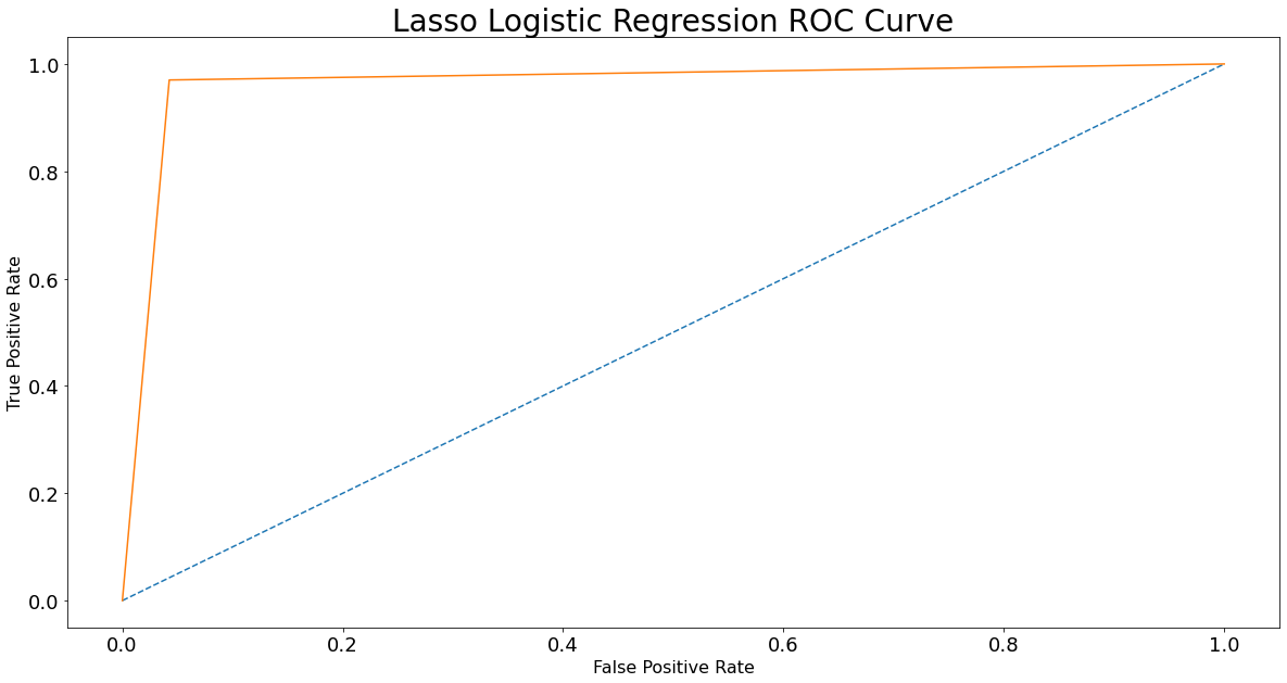
fpr, tpr, thresholds = roc_curve(Y_test, Y_pred)
plt.figure(figsize = (20,10))
plt.plot([0, 1], [0, 1], linestyle = '--')
plt.plot(fpr, tpr)
plt.xlabel('False Positive Rate', fontsize = 16)
plt.ylabel('True Positive Rate', fontsize = 16)
plt.xticks(size = 18)
plt.yticks(size = 18)
plt.title('Lasso Logistic Regression ROC Curve', fontsize = 28)
plt.show();
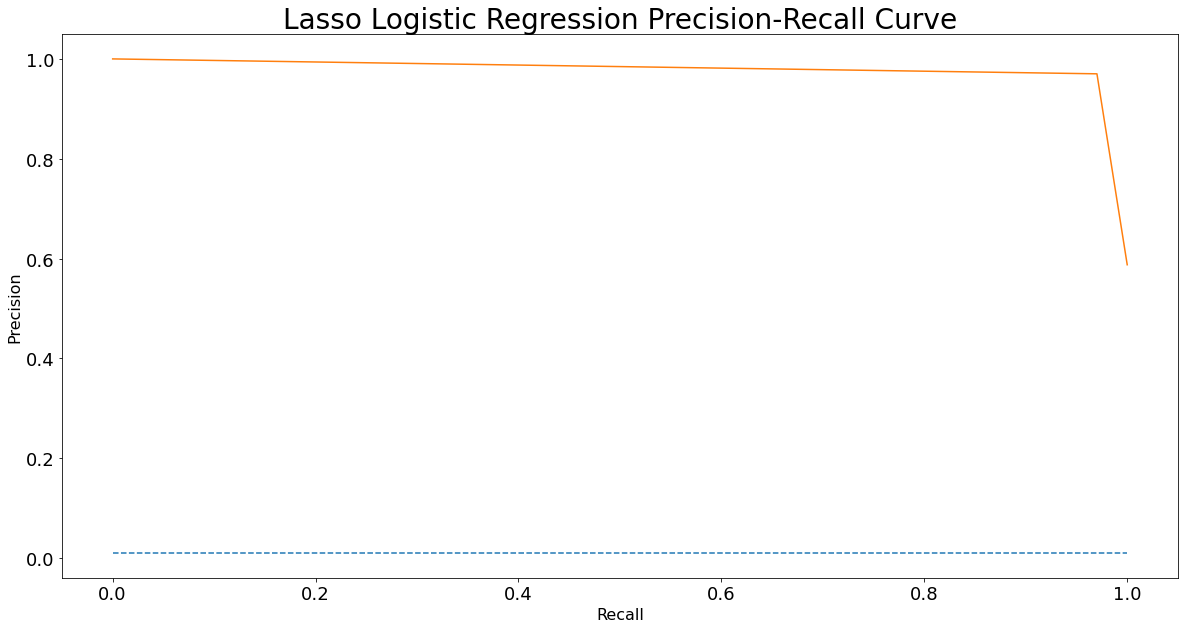
from sklearn.metrics import precision_recall_curve
from sklearn.metrics import average_precision_score
precision, recall, thresholds = precision_recall_curve(Y_test, Y_pred)
plt.figure(figsize = (20,10))
plt.plot([0, 1], [0.01/0.98, 0.01/0.98], linestyle = '--')
plt.plot(recall, precision)
plt.xlabel('Recall', fontsize = 16)
plt.ylabel('Precision', fontsize = 16)
plt.xticks(size = 18)
plt.yticks(size = 18)
plt.title('Lasso Logistic Regression Precision-Recall Curve', fontsize = 28)
plt.show();
len(data.target)
569
sum(data.target)
357
569-357
212
212/569
0.37258347978910367