Part 1#

from IPython.core.interactiveshell import InteractiveShell
InteractiveShell.ast_node_interactivity = "all"

x = 1
y = 2
x
y

Load sample dataset#

from sklearn.datasets import load_iris
from sklearn.datasets import load_diabetes

iris_dataset = load_iris()

iris_dataset

{'data': array([[5.1, 3.5, 1.4, 0.2],
        [4.9, 3. , 1.4, 0.2],
        [4.7, 3.2, 1.3, 0.2],
        [4.6, 3.1, 1.5, 0.2],
        [5. , 3.6, 1.4, 0.2],
        [5.4, 3.9, 1.7, 0.4],
        [4.6, 3.4, 1.4, 0.3],
        [5. , 3.4, 1.5, 0.2],
        [4.4, 2.9, 1.4, 0.2],
        [4.9, 3.1, 1.5, 0.1],
        [5.4, 3.7, 1.5, 0.2],
        [4.8, 3.4, 1.6, 0.2],
        [4.8, 3. , 1.4, 0.1],
        [4.3, 3. , 1.1, 0.1],
        [5.8, 4. , 1.2, 0.2],
        [5.7, 4.4, 1.5, 0.4],
        [5.4, 3.9, 1.3, 0.4],
        [5.1, 3.5, 1.4, 0.3],
        [5.7, 3.8, 1.7, 0.3],
        [5.1, 3.8, 1.5, 0.3],
        [5.4, 3.4, 1.7, 0.2],
        [5.1, 3.7, 1.5, 0.4],
        [4.6, 3.6, 1. , 0.2],
        [5.1, 3.3, 1.7, 0.5],
        [4.8, 3.4, 1.9, 0.2],
        [5. , 3. , 1.6, 0.2],
        [5. , 3.4, 1.6, 0.4],
        [5.2, 3.5, 1.5, 0.2],
        [5.2, 3.4, 1.4, 0.2],
        [4.7, 3.2, 1.6, 0.2],
        [4.8, 3.1, 1.6, 0.2],
        [5.4, 3.4, 1.5, 0.4],
        [5.2, 4.1, 1.5, 0.1],
        [5.5, 4.2, 1.4, 0.2],
        [4.9, 3.1, 1.5, 0.2],
        [5. , 3.2, 1.2, 0.2],
        [5.5, 3.5, 1.3, 0.2],
        [4.9, 3.6, 1.4, 0.1],
        [4.4, 3. , 1.3, 0.2],
        [5.1, 3.4, 1.5, 0.2],
        [5. , 3.5, 1.3, 0.3],
        [4.5, 2.3, 1.3, 0.3],
        [4.4, 3.2, 1.3, 0.2],
        [5. , 3.5, 1.6, 0.6],
        [5.1, 3.8, 1.9, 0.4],
        [4.8, 3. , 1.4, 0.3],
        [5.1, 3.8, 1.6, 0.2],
        [4.6, 3.2, 1.4, 0.2],
        [5.3, 3.7, 1.5, 0.2],
        [5. , 3.3, 1.4, 0.2],
        [7. , 3.2, 4.7, 1.4],
        [6.4, 3.2, 4.5, 1.5],
        [6.9, 3.1, 4.9, 1.5],
        [5.5, 2.3, 4. , 1.3],
        [6.5, 2.8, 4.6, 1.5],
        [5.7, 2.8, 4.5, 1.3],
        [6.3, 3.3, 4.7, 1.6],
        [4.9, 2.4, 3.3, 1. ],
        [6.6, 2.9, 4.6, 1.3],
        [5.2, 2.7, 3.9, 1.4],
        [5. , 2. , 3.5, 1. ],
        [5.9, 3. , 4.2, 1.5],
        [6. , 2.2, 4. , 1. ],
        [6.1, 2.9, 4.7, 1.4],
        [5.6, 2.9, 3.6, 1.3],
        [6.7, 3.1, 4.4, 1.4],
        [5.6, 3. , 4.5, 1.5],
        [5.8, 2.7, 4.1, 1. ],
        [6.2, 2.2, 4.5, 1.5],
        [5.6, 2.5, 3.9, 1.1],
        [5.9, 3.2, 4.8, 1.8],
        [6.1, 2.8, 4. , 1.3],
        [6.3, 2.5, 4.9, 1.5],
        [6.1, 2.8, 4.7, 1.2],
        [6.4, 2.9, 4.3, 1.3],
        [6.6, 3. , 4.4, 1.4],
        [6.8, 2.8, 4.8, 1.4],
        [6.7, 3. , 5. , 1.7],
        [6. , 2.9, 4.5, 1.5],
        [5.7, 2.6, 3.5, 1. ],
        [5.5, 2.4, 3.8, 1.1],
        [5.5, 2.4, 3.7, 1. ],
        [5.8, 2.7, 3.9, 1.2],
        [6. , 2.7, 5.1, 1.6],
        [5.4, 3. , 4.5, 1.5],
        [6. , 3.4, 4.5, 1.6],
        [6.7, 3.1, 4.7, 1.5],
        [6.3, 2.3, 4.4, 1.3],
        [5.6, 3. , 4.1, 1.3],
        [5.5, 2.5, 4. , 1.3],
        [5.5, 2.6, 4.4, 1.2],
        [6.1, 3. , 4.6, 1.4],
        [5.8, 2.6, 4. , 1.2],
        [5. , 2.3, 3.3, 1. ],
        [5.6, 2.7, 4.2, 1.3],
        [5.7, 3. , 4.2, 1.2],
        [5.7, 2.9, 4.2, 1.3],
        [6.2, 2.9, 4.3, 1.3],
        [5.1, 2.5, 3. , 1.1],
        [5.7, 2.8, 4.1, 1.3],
        [6.3, 3.3, 6. , 2.5],
        [5.8, 2.7, 5.1, 1.9],
        [7.1, 3. , 5.9, 2.1],
        [6.3, 2.9, 5.6, 1.8],
        [6.5, 3. , 5.8, 2.2],
        [7.6, 3. , 6.6, 2.1],
        [4.9, 2.5, 4.5, 1.7],
        [7.3, 2.9, 6.3, 1.8],
        [6.7, 2.5, 5.8, 1.8],
        [7.2, 3.6, 6.1, 2.5],
        [6.5, 3.2, 5.1, 2. ],
        [6.4, 2.7, 5.3, 1.9],
        [6.8, 3. , 5.5, 2.1],
        [5.7, 2.5, 5. , 2. ],
        [5.8, 2.8, 5.1, 2.4],
        [6.4, 3.2, 5.3, 2.3],
        [6.5, 3. , 5.5, 1.8],
        [7.7, 3.8, 6.7, 2.2],
        [7.7, 2.6, 6.9, 2.3],
        [6. , 2.2, 5. , 1.5],
        [6.9, 3.2, 5.7, 2.3],
        [5.6, 2.8, 4.9, 2. ],
        [7.7, 2.8, 6.7, 2. ],
        [6.3, 2.7, 4.9, 1.8],
        [6.7, 3.3, 5.7, 2.1],
        [7.2, 3.2, 6. , 1.8],
        [6.2, 2.8, 4.8, 1.8],
        [6.1, 3. , 4.9, 1.8],
        [6.4, 2.8, 5.6, 2.1],
        [7.2, 3. , 5.8, 1.6],
        [7.4, 2.8, 6.1, 1.9],
        [7.9, 3.8, 6.4, 2. ],
        [6.4, 2.8, 5.6, 2.2],
        [6.3, 2.8, 5.1, 1.5],
        [6.1, 2.6, 5.6, 1.4],
        [7.7, 3. , 6.1, 2.3],
        [6.3, 3.4, 5.6, 2.4],
        [6.4, 3.1, 5.5, 1.8],
        [6. , 3. , 4.8, 1.8],
        [6.9, 3.1, 5.4, 2.1],
        [6.7, 3.1, 5.6, 2.4],
        [6.9, 3.1, 5.1, 2.3],
        [5.8, 2.7, 5.1, 1.9],
        [6.8, 3.2, 5.9, 2.3],
        [6.7, 3.3, 5.7, 2.5],
        [6.7, 3. , 5.2, 2.3],
        [6.3, 2.5, 5. , 1.9],
        [6.5, 3. , 5.2, 2. ],
        [6.2, 3.4, 5.4, 2.3],
        [5.9, 3. , 5.1, 1.8]]),
 'target': array([0, 0, 0, 0, 0, 0, 0, 0, 0, 0, 0, 0, 0, 0, 0, 0, 0, 0, 0, 0, 0, 0,
        0, 0, 0, 0, 0, 0, 0, 0, 0, 0, 0, 0, 0, 0, 0, 0, 0, 0, 0, 0, 0, 0,
        0, 0, 0, 0, 0, 0, 1, 1, 1, 1, 1, 1, 1, 1, 1, 1, 1, 1, 1, 1, 1, 1,
        1, 1, 1, 1, 1, 1, 1, 1, 1, 1, 1, 1, 1, 1, 1, 1, 1, 1, 1, 1, 1, 1,
        1, 1, 1, 1, 1, 1, 1, 1, 1, 1, 1, 1, 2, 2, 2, 2, 2, 2, 2, 2, 2, 2,
        2, 2, 2, 2, 2, 2, 2, 2, 2, 2, 2, 2, 2, 2, 2, 2, 2, 2, 2, 2, 2, 2,
        2, 2, 2, 2, 2, 2, 2, 2, 2, 2, 2, 2, 2, 2, 2, 2, 2, 2]),
 'frame': None,
 'target_names': array(['setosa', 'versicolor', 'virginica'], dtype='<U10'),
 'DESCR': '.. _iris_dataset:\n\nIris plants dataset\n--------------------\n\n**Data Set Characteristics:**\n\n    :Number of Instances: 150 (50 in each of three classes)\n    :Number of Attributes: 4 numeric, predictive attributes and the class\n    :Attribute Information:\n        - sepal length in cm\n        - sepal width in cm\n        - petal length in cm\n        - petal width in cm\n        - class:\n                - Iris-Setosa\n                - Iris-Versicolour\n                - Iris-Virginica\n                \n    :Summary Statistics:\n\n    ============== ==== ==== ======= ===== ====================\n                    Min  Max   Mean    SD   Class Correlation\n    ============== ==== ==== ======= ===== ====================\n    sepal length:   4.3  7.9   5.84   0.83    0.7826\n    sepal width:    2.0  4.4   3.05   0.43   -0.4194\n    petal length:   1.0  6.9   3.76   1.76    0.9490  (high!)\n    petal width:    0.1  2.5   1.20   0.76    0.9565  (high!)\n    ============== ==== ==== ======= ===== ====================\n\n    :Missing Attribute Values: None\n    :Class Distribution: 33.3% for each of 3 classes.\n    :Creator: R.A. Fisher\n    :Donor: Michael Marshall (MARSHALL%PLU@io.arc.nasa.gov)\n    :Date: July, 1988\n\nThe famous Iris database, first used by Sir R.A. Fisher. The dataset is taken\nfrom Fisher\'s paper. Note that it\'s the same as in R, but not as in the UCI\nMachine Learning Repository, which has two wrong data points.\n\nThis is perhaps the best known database to be found in the\npattern recognition literature.  Fisher\'s paper is a classic in the field and\nis referenced frequently to this day.  (See Duda & Hart, for example.)  The\ndata set contains 3 classes of 50 instances each, where each class refers to a\ntype of iris plant.  One class is linearly separable from the other 2; the\nlatter are NOT linearly separable from each other.\n\n.. topic:: References\n\n   - Fisher, R.A. "The use of multiple measurements in taxonomic problems"\n     Annual Eugenics, 7, Part II, 179-188 (1936); also in "Contributions to\n     Mathematical Statistics" (John Wiley, NY, 1950).\n   - Duda, R.O., & Hart, P.E. (1973) Pattern Classification and Scene Analysis.\n     (Q327.D83) John Wiley & Sons.  ISBN 0-471-22361-1.  See page 218.\n   - Dasarathy, B.V. (1980) "Nosing Around the Neighborhood: A New System\n     Structure and Classification Rule for Recognition in Partially Exposed\n     Environments".  IEEE Transactions on Pattern Analysis and Machine\n     Intelligence, Vol. PAMI-2, No. 1, 67-71.\n   - Gates, G.W. (1972) "The Reduced Nearest Neighbor Rule".  IEEE Transactions\n     on Information Theory, May 1972, 431-433.\n   - See also: 1988 MLC Proceedings, 54-64.  Cheeseman et al"s AUTOCLASS II\n     conceptual clustering system finds 3 classes in the data.\n   - Many, many more ...',
 'feature_names': ['sepal length (cm)',
  'sepal width (cm)',
  'petal length (cm)',
  'petal width (cm)'],
 'filename': 'iris.csv',
 'data_module': 'sklearn.datasets.data'}

print(iris_dataset.DESCR)

.. _iris_dataset:

Iris plants dataset
--------------------

**Data Set Characteristics:**

    :Number of Instances: 150 (50 in each of three classes)
    :Number of Attributes: 4 numeric, predictive attributes and the class
    :Attribute Information:
        - sepal length in cm
        - sepal width in cm
        - petal length in cm
        - petal width in cm
        - class:
                - Iris-Setosa
                - Iris-Versicolour
                - Iris-Virginica
                
    :Summary Statistics:

    ============== ==== ==== ======= ===== ====================
                    Min  Max   Mean    SD   Class Correlation
    ============== ==== ==== ======= ===== ====================
    sepal length:   4.3  7.9   5.84   0.83    0.7826
    sepal width:    2.0  4.4   3.05   0.43   -0.4194
    petal length:   1.0  6.9   3.76   1.76    0.9490  (high!)
    petal width:    0.1  2.5   1.20   0.76    0.9565  (high!)
    ============== ==== ==== ======= ===== ====================

    :Missing Attribute Values: None
    :Class Distribution: 33.3% for each of 3 classes.
    :Creator: R.A. Fisher
    :Donor: Michael Marshall (MARSHALL%PLU@io.arc.nasa.gov)
    :Date: July, 1988

The famous Iris database, first used by Sir R.A. Fisher. The dataset is taken
from Fisher's paper. Note that it's the same as in R, but not as in the UCI
Machine Learning Repository, which has two wrong data points.

This is perhaps the best known database to be found in the
pattern recognition literature.  Fisher's paper is a classic in the field and
is referenced frequently to this day.  (See Duda & Hart, for example.)  The
data set contains 3 classes of 50 instances each, where each class refers to a
type of iris plant.  One class is linearly separable from the other 2; the
latter are NOT linearly separable from each other.

.. topic:: References

   - Fisher, R.A. "The use of multiple measurements in taxonomic problems"
     Annual Eugenics, 7, Part II, 179-188 (1936); also in "Contributions to
     Mathematical Statistics" (John Wiley, NY, 1950).
   - Duda, R.O., & Hart, P.E. (1973) Pattern Classification and Scene Analysis.
     (Q327.D83) John Wiley & Sons.  ISBN 0-471-22361-1.  See page 218.
   - Dasarathy, B.V. (1980) "Nosing Around the Neighborhood: A New System
     Structure and Classification Rule for Recognition in Partially Exposed
     Environments".  IEEE Transactions on Pattern Analysis and Machine
     Intelligence, Vol. PAMI-2, No. 1, 67-71.
   - Gates, G.W. (1972) "The Reduced Nearest Neighbor Rule".  IEEE Transactions
     on Information Theory, May 1972, 431-433.
   - See also: 1988 MLC Proceedings, 54-64.  Cheeseman et al"s AUTOCLASS II
     conceptual clustering system finds 3 classes in the data.
   - Many, many more ...

iris_dataset.data

array([[5.1, 3.5, 1.4, 0.2],
       [4.9, 3. , 1.4, 0.2],
       [4.7, 3.2, 1.3, 0.2],
       [4.6, 3.1, 1.5, 0.2],
       [5. , 3.6, 1.4, 0.2],
       [5.4, 3.9, 1.7, 0.4],
       [4.6, 3.4, 1.4, 0.3],
       [5. , 3.4, 1.5, 0.2],
       [4.4, 2.9, 1.4, 0.2],
       [4.9, 3.1, 1.5, 0.1],
       [5.4, 3.7, 1.5, 0.2],
       [4.8, 3.4, 1.6, 0.2],
       [4.8, 3. , 1.4, 0.1],
       [4.3, 3. , 1.1, 0.1],
       [5.8, 4. , 1.2, 0.2],
       [5.7, 4.4, 1.5, 0.4],
       [5.4, 3.9, 1.3, 0.4],
       [5.1, 3.5, 1.4, 0.3],
       [5.7, 3.8, 1.7, 0.3],
       [5.1, 3.8, 1.5, 0.3],
       [5.4, 3.4, 1.7, 0.2],
       [5.1, 3.7, 1.5, 0.4],
       [4.6, 3.6, 1. , 0.2],
       [5.1, 3.3, 1.7, 0.5],
       [4.8, 3.4, 1.9, 0.2],
       [5. , 3. , 1.6, 0.2],
       [5. , 3.4, 1.6, 0.4],
       [5.2, 3.5, 1.5, 0.2],
       [5.2, 3.4, 1.4, 0.2],
       [4.7, 3.2, 1.6, 0.2],
       [4.8, 3.1, 1.6, 0.2],
       [5.4, 3.4, 1.5, 0.4],
       [5.2, 4.1, 1.5, 0.1],
       [5.5, 4.2, 1.4, 0.2],
       [4.9, 3.1, 1.5, 0.2],
       [5. , 3.2, 1.2, 0.2],
       [5.5, 3.5, 1.3, 0.2],
       [4.9, 3.6, 1.4, 0.1],
       [4.4, 3. , 1.3, 0.2],
       [5.1, 3.4, 1.5, 0.2],
       [5. , 3.5, 1.3, 0.3],
       [4.5, 2.3, 1.3, 0.3],
       [4.4, 3.2, 1.3, 0.2],
       [5. , 3.5, 1.6, 0.6],
       [5.1, 3.8, 1.9, 0.4],
       [4.8, 3. , 1.4, 0.3],
       [5.1, 3.8, 1.6, 0.2],
       [4.6, 3.2, 1.4, 0.2],
       [5.3, 3.7, 1.5, 0.2],
       [5. , 3.3, 1.4, 0.2],
       [7. , 3.2, 4.7, 1.4],
       [6.4, 3.2, 4.5, 1.5],
       [6.9, 3.1, 4.9, 1.5],
       [5.5, 2.3, 4. , 1.3],
       [6.5, 2.8, 4.6, 1.5],
       [5.7, 2.8, 4.5, 1.3],
       [6.3, 3.3, 4.7, 1.6],
       [4.9, 2.4, 3.3, 1. ],
       [6.6, 2.9, 4.6, 1.3],
       [5.2, 2.7, 3.9, 1.4],
       [5. , 2. , 3.5, 1. ],
       [5.9, 3. , 4.2, 1.5],
       [6. , 2.2, 4. , 1. ],
       [6.1, 2.9, 4.7, 1.4],
       [5.6, 2.9, 3.6, 1.3],
       [6.7, 3.1, 4.4, 1.4],
       [5.6, 3. , 4.5, 1.5],
       [5.8, 2.7, 4.1, 1. ],
       [6.2, 2.2, 4.5, 1.5],
       [5.6, 2.5, 3.9, 1.1],
       [5.9, 3.2, 4.8, 1.8],
       [6.1, 2.8, 4. , 1.3],
       [6.3, 2.5, 4.9, 1.5],
       [6.1, 2.8, 4.7, 1.2],
       [6.4, 2.9, 4.3, 1.3],
       [6.6, 3. , 4.4, 1.4],
       [6.8, 2.8, 4.8, 1.4],
       [6.7, 3. , 5. , 1.7],
       [6. , 2.9, 4.5, 1.5],
       [5.7, 2.6, 3.5, 1. ],
       [5.5, 2.4, 3.8, 1.1],
       [5.5, 2.4, 3.7, 1. ],
       [5.8, 2.7, 3.9, 1.2],
       [6. , 2.7, 5.1, 1.6],
       [5.4, 3. , 4.5, 1.5],
       [6. , 3.4, 4.5, 1.6],
       [6.7, 3.1, 4.7, 1.5],
       [6.3, 2.3, 4.4, 1.3],
       [5.6, 3. , 4.1, 1.3],
       [5.5, 2.5, 4. , 1.3],
       [5.5, 2.6, 4.4, 1.2],
       [6.1, 3. , 4.6, 1.4],
       [5.8, 2.6, 4. , 1.2],
       [5. , 2.3, 3.3, 1. ],
       [5.6, 2.7, 4.2, 1.3],
       [5.7, 3. , 4.2, 1.2],
       [5.7, 2.9, 4.2, 1.3],
       [6.2, 2.9, 4.3, 1.3],
       [5.1, 2.5, 3. , 1.1],
       [5.7, 2.8, 4.1, 1.3],
       [6.3, 3.3, 6. , 2.5],
       [5.8, 2.7, 5.1, 1.9],
       [7.1, 3. , 5.9, 2.1],
       [6.3, 2.9, 5.6, 1.8],
       [6.5, 3. , 5.8, 2.2],
       [7.6, 3. , 6.6, 2.1],
       [4.9, 2.5, 4.5, 1.7],
       [7.3, 2.9, 6.3, 1.8],
       [6.7, 2.5, 5.8, 1.8],
       [7.2, 3.6, 6.1, 2.5],
       [6.5, 3.2, 5.1, 2. ],
       [6.4, 2.7, 5.3, 1.9],
       [6.8, 3. , 5.5, 2.1],
       [5.7, 2.5, 5. , 2. ],
       [5.8, 2.8, 5.1, 2.4],
       [6.4, 3.2, 5.3, 2.3],
       [6.5, 3. , 5.5, 1.8],
       [7.7, 3.8, 6.7, 2.2],
       [7.7, 2.6, 6.9, 2.3],
       [6. , 2.2, 5. , 1.5],
       [6.9, 3.2, 5.7, 2.3],
       [5.6, 2.8, 4.9, 2. ],
       [7.7, 2.8, 6.7, 2. ],
       [6.3, 2.7, 4.9, 1.8],
       [6.7, 3.3, 5.7, 2.1],
       [7.2, 3.2, 6. , 1.8],
       [6.2, 2.8, 4.8, 1.8],
       [6.1, 3. , 4.9, 1.8],
       [6.4, 2.8, 5.6, 2.1],
       [7.2, 3. , 5.8, 1.6],
       [7.4, 2.8, 6.1, 1.9],
       [7.9, 3.8, 6.4, 2. ],
       [6.4, 2.8, 5.6, 2.2],
       [6.3, 2.8, 5.1, 1.5],
       [6.1, 2.6, 5.6, 1.4],
       [7.7, 3. , 6.1, 2.3],
       [6.3, 3.4, 5.6, 2.4],
       [6.4, 3.1, 5.5, 1.8],
       [6. , 3. , 4.8, 1.8],
       [6.9, 3.1, 5.4, 2.1],
       [6.7, 3.1, 5.6, 2.4],
       [6.9, 3.1, 5.1, 2.3],
       [5.8, 2.7, 5.1, 1.9],
       [6.8, 3.2, 5.9, 2.3],
       [6.7, 3.3, 5.7, 2.5],
       [6.7, 3. , 5.2, 2.3],
       [6.3, 2.5, 5. , 1.9],
       [6.5, 3. , 5.2, 2. ],
       [6.2, 3.4, 5.4, 2.3],
       [5.9, 3. , 5.1, 1.8]])

iris_dataset.target

array([0, 0, 0, 0, 0, 0, 0, 0, 0, 0, 0, 0, 0, 0, 0, 0, 0, 0, 0, 0, 0, 0,
       0, 0, 0, 0, 0, 0, 0, 0, 0, 0, 0, 0, 0, 0, 0, 0, 0, 0, 0, 0, 0, 0,
       0, 0, 0, 0, 0, 0, 1, 1, 1, 1, 1, 1, 1, 1, 1, 1, 1, 1, 1, 1, 1, 1,
       1, 1, 1, 1, 1, 1, 1, 1, 1, 1, 1, 1, 1, 1, 1, 1, 1, 1, 1, 1, 1, 1,
       1, 1, 1, 1, 1, 1, 1, 1, 1, 1, 1, 1, 2, 2, 2, 2, 2, 2, 2, 2, 2, 2,
       2, 2, 2, 2, 2, 2, 2, 2, 2, 2, 2, 2, 2, 2, 2, 2, 2, 2, 2, 2, 2, 2,
       2, 2, 2, 2, 2, 2, 2, 2, 2, 2, 2, 2, 2, 2, 2, 2, 2, 2])

iris_dataset.target_names

array(['setosa', 'versicolor', 'virginica'], dtype='<U10')

diabetes =  load_diabetes()
print(diabetes.DESCR)

.. _diabetes_dataset:

Diabetes dataset
----------------

Ten baseline variables, age, sex, body mass index, average blood
pressure, and six blood serum measurements were obtained for each of n =
442 diabetes patients, as well as the response of interest, a
quantitative measure of disease progression one year after baseline.

**Data Set Characteristics:**

  :Number of Instances: 442

  :Number of Attributes: First 10 columns are numeric predictive values

  :Target: Column 11 is a quantitative measure of disease progression one year after baseline

  :Attribute Information:
      - age     age in years
      - sex
      - bmi     body mass index
      - bp      average blood pressure
      - s1      tc, total serum cholesterol
      - s2      ldl, low-density lipoproteins
      - s3      hdl, high-density lipoproteins
      - s4      tch, total cholesterol / HDL
      - s5      ltg, possibly log of serum triglycerides level
      - s6      glu, blood sugar level

Note: Each of these 10 feature variables have been mean centered and scaled by the standard deviation times `n_samples` (i.e. the sum of squares of each column totals 1).

Source URL:
https://www4.stat.ncsu.edu/~boos/var.select/diabetes.html

For more information see:
Bradley Efron, Trevor Hastie, Iain Johnstone and Robert Tibshirani (2004) "Least Angle Regression," Annals of Statistics (with discussion), 407-499.
(https://web.stanford.edu/~hastie/Papers/LARS/LeastAngle_2002.pdf)

import pandas as pd

pd.DataFrame(diabetes.data, columns=diabetes.feature_names)

	age	sex	bmi	bp	s1	s2	s3	s4	s5	s6
0	0.038076	0.050680	0.061696	0.021872	-0.044223	-0.034821	-0.043401	-0.002592	0.019908	-0.017646
1	-0.001882	-0.044642	-0.051474	-0.026328	-0.008449	-0.019163	0.074412	-0.039493	-0.068330	-0.092204
2	0.085299	0.050680	0.044451	-0.005671	-0.045599	-0.034194	-0.032356	-0.002592	0.002864	-0.025930
3	-0.089063	-0.044642	-0.011595	-0.036656	0.012191	0.024991	-0.036038	0.034309	0.022692	-0.009362
4	0.005383	-0.044642	-0.036385	0.021872	0.003935	0.015596	0.008142	-0.002592	-0.031991	-0.046641
...	...	...	...	...	...	...	...	...	...	...
437	0.041708	0.050680	0.019662	0.059744	-0.005697	-0.002566	-0.028674	-0.002592	0.031193	0.007207
438	-0.005515	0.050680	-0.015906	-0.067642	0.049341	0.079165	-0.028674	0.034309	-0.018118	0.044485
439	0.041708	0.050680	-0.015906	0.017282	-0.037344	-0.013840	-0.024993	-0.011080	-0.046879	0.015491
440	-0.045472	-0.044642	0.039062	0.001215	0.016318	0.015283	-0.028674	0.026560	0.044528	-0.025930
441	-0.045472	-0.044642	-0.073030	-0.081414	0.083740	0.027809	0.173816	-0.039493	-0.004220	0.003064

442 rows × 10 columns

print(diabetes.DESCR)

.. _diabetes_dataset:

Diabetes dataset
----------------

Ten baseline variables, age, sex, body mass index, average blood
pressure, and six blood serum measurements were obtained for each of n =
442 diabetes patients, as well as the response of interest, a
quantitative measure of disease progression one year after baseline.

**Data Set Characteristics:**

  :Number of Instances: 442

  :Number of Attributes: First 10 columns are numeric predictive values

  :Target: Column 11 is a quantitative measure of disease progression one year after baseline

  :Attribute Information:
      - age     age in years
      - sex
      - bmi     body mass index
      - bp      average blood pressure
      - s1      tc, total serum cholesterol
      - s2      ldl, low-density lipoproteins
      - s3      hdl, high-density lipoproteins
      - s4      tch, total cholesterol / HDL
      - s5      ltg, possibly log of serum triglycerides level
      - s6      glu, blood sugar level

Note: Each of these 10 feature variables have been mean centered and scaled by the standard deviation times `n_samples` (i.e. the sum of squares of each column totals 1).

Source URL:
https://www4.stat.ncsu.edu/~boos/var.select/diabetes.html

For more information see:
Bradley Efron, Trevor Hastie, Iain Johnstone and Robert Tibshirani (2004) "Least Angle Regression," Annals of Statistics (with discussion), 407-499.
(https://web.stanford.edu/~hastie/Papers/LARS/LeastAngle_2002.pdf)

Loading data from the web#

import sklearn
from sklearn.datasets import fetch_california_housing

houses = fetch_california_housing()

print(houses.DESCR)

.. _california_housing_dataset:

California Housing dataset
--------------------------

**Data Set Characteristics:**

    :Number of Instances: 20640

    :Number of Attributes: 8 numeric, predictive attributes and the target

    :Attribute Information:
        - MedInc        median income in block group
        - HouseAge      median house age in block group
        - AveRooms      average number of rooms per household
        - AveBedrms     average number of bedrooms per household
        - Population    block group population
        - AveOccup      average number of household members
        - Latitude      block group latitude
        - Longitude     block group longitude

    :Missing Attribute Values: None

This dataset was obtained from the StatLib repository.
https://www.dcc.fc.up.pt/~ltorgo/Regression/cal_housing.html

The target variable is the median house value for California districts,
expressed in hundreds of thousands of dollars ($100,000).

This dataset was derived from the 1990 U.S. census, using one row per census
block group. A block group is the smallest geographical unit for which the U.S.
Census Bureau publishes sample data (a block group typically has a population
of 600 to 3,000 people).

An household is a group of people residing within a home. Since the average
number of rooms and bedrooms in this dataset are provided per household, these
columns may take surpinsingly large values for block groups with few households
and many empty houses, such as vacation resorts.

It can be downloaded/loaded using the
:func:`sklearn.datasets.fetch_california_housing` function.

.. topic:: References

    - Pace, R. Kelley and Ronald Barry, Sparse Spatial Autoregressions,
      Statistics and Probability Letters, 33 (1997) 291-297

houses.data.shape
houses.feature_names
pd.DataFrame(houses.data, columns=houses.feature_names)

(20640, 8)

['MedInc',
 'HouseAge',
 'AveRooms',
 'AveBedrms',
 'Population',
 'AveOccup',
 'Latitude',
 'Longitude']

	MedInc	HouseAge	AveRooms	AveBedrms	Population	AveOccup	Latitude	Longitude
0	8.3252	41.0	6.984127	1.023810	322.0	2.555556	37.88	-122.23
1	8.3014	21.0	6.238137	0.971880	2401.0	2.109842	37.86	-122.22
2	7.2574	52.0	8.288136	1.073446	496.0	2.802260	37.85	-122.24
3	5.6431	52.0	5.817352	1.073059	558.0	2.547945	37.85	-122.25
4	3.8462	52.0	6.281853	1.081081	565.0	2.181467	37.85	-122.25
...	...	...	...	...	...	...	...	...
20635	1.5603	25.0	5.045455	1.133333	845.0	2.560606	39.48	-121.09
20636	2.5568	18.0	6.114035	1.315789	356.0	3.122807	39.49	-121.21
20637	1.7000	17.0	5.205543	1.120092	1007.0	2.325635	39.43	-121.22
20638	1.8672	18.0	5.329513	1.171920	741.0	2.123209	39.43	-121.32
20639	2.3886	16.0	5.254717	1.162264	1387.0	2.616981	39.37	-121.24

20640 rows × 8 columns

diabetes.data.shape

(442, 10)

Generate dataset#

from sklearn.datasets import make_regression
x,y = make_regression(n_samples=100, n_features=5, n_targets=1, noise=0.005)

pd.DataFrame(y)

	0
0	-56.878301
1	157.174068
2	-20.096663
3	-7.563574
4	27.367709
...	...
95	-31.741801
96	8.639267
97	-68.500575
98	-62.879911
99	-10.838747

100 rows × 1 columns

pd.DataFrame(x)

	0	1	2	3	4
0	0.161720	0.091843	0.095730	-1.913515	0.140882
1	0.272338	1.283241	0.529606	0.973450	0.628376
2	-0.251843	-0.157911	1.327633	-1.302578	0.441988
3	0.117548	0.301254	-0.043708	0.134207	-0.478126
4	-1.040602	0.352708	0.360921	-1.766644	1.595943
...	...	...	...	...	...
95	0.558344	-0.631148	-1.208268	-0.654117	0.435893
96	0.971506	-0.573440	0.403751	0.455868	-0.173494
97	-0.506183	-0.375183	1.588506	-0.896150	-0.352137
98	0.186767	0.093694	-1.776359	0.301386	-0.949856
99	-0.102822	-0.613607	-1.191659	2.246375	-0.792975

100 rows × 5 columns

import seaborn as sns
sns.set(color_codes=True)
sns.regplot(x=x, y=y);

---------------------------------------------------------------------------
ValueError                                Traceback (most recent call last)
Input In [21], in <cell line: 3>()
      1 import seaborn as sns
      2 sns.set(color_codes=True)
----> 3 sns.regplot(x=x, y=y)

File ~/anaconda3/lib/python3.9/site-packages/seaborn/_decorators.py:46, in _deprecate_positional_args.<locals>.inner_f(*args, **kwargs)
     36     warnings.warn(
     37         "Pass the following variable{} as {}keyword arg{}: {}. "
     38         "From version 0.12, the only valid positional argument "
   (...)
     43         FutureWarning
     44     )
     45 kwargs.update({k: arg for k, arg in zip(sig.parameters, args)})
---> 46 return f(**kwargs)

File ~/anaconda3/lib/python3.9/site-packages/seaborn/regression.py:851, in regplot(x, y, data, x_estimator, x_bins, x_ci, scatter, fit_reg, ci, n_boot, units, seed, order, logistic, lowess, robust, logx, x_partial, y_partial, truncate, dropna, x_jitter, y_jitter, label, color, marker, scatter_kws, line_kws, ax)
    837 @_deprecate_positional_args
    838 def regplot(
    839     *,
   (...)
    848     scatter_kws=None, line_kws=None, ax=None
    849 ):
--> 851     plotter = _RegressionPlotter(x, y, data, x_estimator, x_bins, x_ci,
    852                                  scatter, fit_reg, ci, n_boot, units, seed,
    853                                  order, logistic, lowess, robust, logx,
    854                                  x_partial, y_partial, truncate, dropna,
    855                                  x_jitter, y_jitter, color, label)
    857     if ax is None:
    858         ax = plt.gca()

File ~/anaconda3/lib/python3.9/site-packages/seaborn/regression.py:109, in _RegressionPlotter.__init__(self, x, y, data, x_estimator, x_bins, x_ci, scatter, fit_reg, ci, n_boot, units, seed, order, logistic, lowess, robust, logx, x_partial, y_partial, truncate, dropna, x_jitter, y_jitter, color, label)
    106     raise ValueError("Mutually exclusive regression options.")
    108 # Extract the data vals from the arguments or passed dataframe
--> 109 self.establish_variables(data, x=x, y=y, units=units,
    110                          x_partial=x_partial, y_partial=y_partial)
    112 # Drop null observations
    113 if dropna:

File ~/anaconda3/lib/python3.9/site-packages/seaborn/regression.py:55, in _LinearPlotter.establish_variables(self, data, **kws)
     53 if np.ndim(vector) > 1:
     54     err = "regplot inputs must be 1d"
---> 55     raise ValueError(err)
     56 setattr(self, var, vector)

ValueError: regplot inputs must be 1d

Load data from openml.org #

from sklearn.datasets import fetch_openml

mice = fetch_openml(name='miceprotein')

print(mice.target)

     c-CS-m
     c-CS-m
     c-CS-m
     c-CS-m
     c-CS-m
         ...  
  t-SC-s
  t-SC-s
  t-SC-s
  t-SC-s
  t-SC-s
Name: class, Length: 1080, dtype: category
Categories (8, object): ['c-CS-m', 'c-CS-s', 'c-SC-m', 'c-SC-s', 't-CS-m', 't-CS-s', 't-SC-m', 't-SC-s']

import numpy as np

d = np.random.rand(3,10)

d.shape

mice.data.shape

print(mice.DESCR)

mice.target_names

import pandas as pd

5.3. Preprocessing data#

Standardization, or mean removal and variance scaling#

Standardization of datasets is a common requirement for many machine learning estimators implemented in scikit-learn; they might behave badly if the individual features do not more or less look like standard normally distributed data: Gaussian with zero mean and unit variance.

In practice we often ignore the shape of the distribution and just transform the data to center it by removing the mean value of each feature, then scale it by dividing non-constant features by their standard deviation.

from IPython.display import display
from sklearn import preprocessing
import numpy as np
X_train = np.array([[ 1., -1.,  2.],
                    [ 2.,  0.,  0.],
                    [ 0.,  1., -1.]])

df = pd.DataFrame(X_train)
display(df)

X_scaled = preprocessing.scale(df)

X_scaled      

#rows are different patients/subjects/flowers
# columns are various features of the patients/subjects/flowers

	0	1	2
0	1.0	-1.0	2.0
1	2.0	0.0	0.0
2	0.0	1.0	-1.0

array([[ 0.        , -1.22474487,  1.33630621],
       [ 1.22474487,  0.        , -0.26726124],
       [-1.22474487,  1.22474487, -1.06904497]])

df.describe()

	0	1	2
count	3.0	3.0	3.000000
mean	1.0	0.0	0.333333
std	1.0	1.0	1.527525
min	0.0	-1.0	-1.000000
25%	0.5	-0.5	-0.500000
50%	1.0	0.0	0.000000
75%	1.5	0.5	1.000000
max	2.0	1.0	2.000000

sum([0.        , -1.22474487,  1.33630621])

0.11156133999999995

idata = iris_dataset.data
id_scaled = preprocessing.scale(idata)
idata.mean(axis=0)
id_scaled.mean(axis=0)
id_scaled.var(axis=0)

array([5.84333333, 3.05733333, 3.758     , 1.19933333])

array([-1.69031455e-15, -1.84297022e-15, -1.69864123e-15, -1.40924309e-15])

array([1., 1., 1., 1.])

X_train.mean(axis=0)
X_scaled.mean(axis=0)

array([1.        , 0.        , 0.33333333])

array([0., 0., 0.])

X_scaled.std(axis=0)

X_scaled.mean(axis=1)

X_scaled.std(axis=1)

Can save scaling and apply to testing data#

scaler = preprocessing.StandardScaler().fit(X_train)
scaler                         
scaler.transform(X_train)      

StandardScaler()

array([[ 0.        , -1.22474487,  1.33630621],
       [ 1.22474487,  0.        , -0.26726124],
       [-1.22474487,  1.22474487, -1.06904497]])

scaler.get_params

{'copy': True, 'with_mean': True, 'with_std': True}

X_test = [[-1., 1., 0.]]
scaler.transform(X_test)  

array([[-2.44948974,  1.22474487, -0.26726124]])

Scaling features to a range#

X_train = np.array([[ 1., -1.,  2.],
                    [ 2.,  0.,  0.],
                    [ 0.,  1., -1.]])

min_max_scaler = preprocessing.MinMaxScaler()
X_train_minmax = min_max_scaler.fit_transform(X_train)
X_train_minmax

array([[0.5       , 0.        , 1.        ],
       [1.        , 0.5       , 0.33333333],
       [0.        , 1.        , 0.        ]])

X_test = np.array([[-3., -1.,  4.]])
X_test_minmax = min_max_scaler.transform(X_test)
X_test_minmax

array([[-1.5       ,  0.        ,  1.66666667]])

Pre-processing data - Non-linear transformation#

import pandas as pd
%matplotlib inline
df = pd.read_csv('international-airline-passengers.csv')
display(df)

	date	passengers
0	1949-01	112.0
1	1949-02	118.0
2	1949-03	132.0
3	1949-04	129.0
4	1949-05	121.0
...	...	...
140	1960-09	508.0
141	1960-10	461.0
142	1960-11	390.0
143	1960-12	432.0
144	International airline passengers: monthly tota...	NaN

145 rows × 2 columns

df.keys()

Index(['date', 'passengers'], dtype='object')

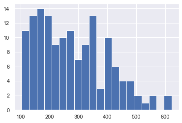
df['passengers'].hist(bins=20)

<AxesSubplot:>

import numpy as np
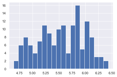
df['passengers'] = np.log(df['passengers'])
df['passengers'].hist(bins=20)

<AxesSubplot:>

5.3.3. Normalization#

from sklearn import preprocessing
X = [[ 1., -1.,  2.],
     [ 2.,  0.,  0.],
     [ 0.,  1., -1.]]
X_normalized = preprocessing.normalize(X, norm='l1')

X_normalized   
# http://www.chioka.in/differences-between-the-l1-norm-and-the-l2-norm-least-absolute-deviations-and-least-squares/

array([[ 0.25, -0.25,  0.5 ],
       [ 1.  ,  0.  ,  0.  ],
       [ 0.  ,  0.5 , -0.5 ]])

Can save the normalization for future use#

normalizer = preprocessing.Normalizer().fit(X)  # fit does nothing
normalizer

Normalizer()

normalizer.transform(X)    

array([[ 0.40824829, -0.40824829,  0.81649658],
       [ 1.        ,  0.        ,  0.        ],
       [ 0.        ,  0.70710678, -0.70710678]])

tmp = normalizer.transform([[2.,  1., 0.]]) 

tmp

array([[0.89442719, 0.4472136 , 0.        ]])

tmp.mean()

0.4472135954999579

(tmp*tmp).sum()

0.9999999999999999

Preprocessing data - Encoding#

from sklearn import preprocessing
enc = preprocessing.OrdinalEncoder()
X = [['male', 'from US', 'uses Safari'], 
     ['female', 'from Europe', 'uses Firefox']]
enc.fit(X)  

OrdinalEncoder()

enc.transform([['female', 'from US', 'uses Safari']])

array([[0., 1., 1.]])

enc.transform([['male', 'from Europe', 'uses Safari']])

array([[1., 0., 1.]])

enc.transform([['female', 'from Europe', 'uses Firefox']])

array([[0., 0., 0.]])

genders = ['female', 'male']
locations = ['from Africa', 'from Asia', 'from Europe', 'from US']
browsers = ['uses Chrome', 'uses Firefox', 'uses IE', 'uses Safari']
enc = preprocessing.OneHotEncoder(categories=[genders, locations, browsers])
X = [['male', 'from US', 'uses Safari'], ['female', 'from Europe', 'uses Firefox']]
enc.fit(X) 
enc.categories_

OneHotEncoder(categories=[['female', 'male'],
                          ['from Africa', 'from Asia', 'from Europe',
                           'from US'],
                          ['uses Chrome', 'uses Firefox', 'uses IE',
                           'uses Safari']])

[array(['female', 'male'], dtype=object),
 array(['from Africa', 'from Asia', 'from Europe', 'from US'], dtype=object),
 array(['uses Chrome', 'uses Firefox', 'uses IE', 'uses Safari'],
       dtype=object)]

enc.transform([['male', 'from US', 'uses Safari']])

tmp = enc.transform([['female', 'from Asia', 'uses Chrome'],
                    ['male', 'from Europe', 'uses Safari']]).toarray()
tmp

array([[1., 0., 0., 1., 0., 0., 1., 0., 0., 0.],
       [0., 1., 0., 0., 1., 0., 0., 0., 0., 1.]])

[0, 1, 0, 0, 1, 0, 0, 0, 0, 1]

[0, 1, 0, 0, 1, 0, 0, 0, 0, 1]

enc.inverse_transform(tmp)

array([['female', 'from Asia', 'uses Chrome'],
       ['male', 'from Europe', 'uses Safari']], dtype=object)

5.3.5. Discretization#

Discretization (otherwise known as quantization or binning) provides a way to partition continuous features into discrete values. Certain datasets with continuous features may benefit from discretization, because discretization can transform the dataset of continuous attributes to one with only nominal attributes.

One-hot encoded discretized features can make a model more expressive, while maintaining interpretability. For instance, pre-processing with a discretizer can introduce nonlinearity to linear models.

X = np.array([[ -3., 5., 15 ],
              [  0., 6., 14 ],
              [  6., 3., 11 ]])
est = preprocessing.KBinsDiscretizer(n_bins=[3, 2, 4], encode='ordinal').fit(X)

est.transform(X)

array([[0., 1., 3.],
       [1., 1., 2.],
       [2., 0., 0.]])

#https://scikit-learn.org/stable/modules/preprocessing.html#k-bins-discretization

5.4.2. Univariate feature imputation#

# Example 1
import numpy as np
from sklearn.impute import SimpleImputer
imp = SimpleImputer(missing_values=np.nan, strategy='mean')
orig_data = [[1, 2],
         [np.nan, 3], 
         [7, 6]]
imp.fit(orig_data)  


imp.transform(orig_data)

SimpleImputer()

array([[1., 2.],
       [4., 3.],
       [7., 6.]])

X = [[np.nan, 2], 
     [6, np.nan], 
     [7, 6]]
print(imp.transform(X))      

[[4.         2.        ]
 [6.         3.66666667]
 [7.         6.        ]]

11/3

3.6666666666666665

import pandas as pd
df = pd.DataFrame([["a", "x"],
                   [np.nan, "w"],
                   ["a", np.nan],
                   ["b", "y"]], dtype="category")

imp = SimpleImputer(strategy="most_frequent")
print(imp.fit_transform(df)) 

[['a' 'x']
 ['a' 'w']
 ['a' 'w']
 ['b' 'y']]

import pandas as pd
df = pd.DataFrame([["a", "x"],
                   [np.nan, "y"],
                   ["c", np.nan],
                   ["b", "y"]], dtype="category")

imp = SimpleImputer(strategy="most_frequent")
print(imp.fit_transform(df)) 

[['a' 'x']
 ['a' 'y']
 ['c' 'y']
 ['b' 'y']]

Splitting data into Train and Test#

import numpy as np
from sklearn.model_selection import train_test_split
X, y = np.arange(10).reshape((5, 2)), [0, 1, 0, 0, 1]
X
list(y)
# X -- feature
# y -- label

array([[0, 1],
       [2, 3],
       [4, 5],
       [6, 7],
       [8, 9]])

[0, 1, 0, 0, 1]

X_train, X_test, y_train, y_test = train_test_split(X, y, test_size=0.2)

X_train

y_train

X_test

y_test

array([[4, 5],
       [2, 3],
       [0, 1],
       [8, 9]])

[0, 1, 0, 1]

array([[6, 7]])

[0]

X_train, X_test, y_train, y_test = train_test_split(
    X, y, test_size=0.40, random_state=43)

X_train

y_train

X_test

y_test

array([[2, 3],
       [0, 1],
       [8, 9]])

[1, 0, 1]

array([[6, 7],
       [4, 5]])

[0, 0]

X_train, X_test, y_train, y_test = train_test_split(
    X, y, test_size=0.33, random_state=42)

X_train

y_train

X_test

y_test

array([[4, 5],
       [0, 1],
       [6, 7]])

[0, 0, 0]

array([[2, 3],
       [8, 9]])

[1, 1]

X_train, X_test, y_train, y_test = train_test_split(
    X, y, test_size=0.33, random_state=np.random)

X_train

y_train

X_test

y_test

array([[6, 7],
       [8, 9],
       [4, 5]])

[0, 1, 0]

array([[0, 1],
       [2, 3]])

[0, 1]

X_train, X_test, y_train, y_test = train_test_split(
    X, y, test_size=0.33, random_state=np.random)

X_train

y_train

X_test

y_test

array([[0, 1],
       [6, 7],
       [8, 9]])

[0, 0, 1]

array([[2, 3],
       [4, 5]])

[1, 0]

import pandas as pd
from sklearn import datasets, linear_model
from sklearn.model_selection import train_test_split
from matplotlib import pyplot as plt

diabetes = datasets.load_diabetes()
diabetes.data.shape

(442, 10)

feature_names = diabetes.feature_names
feature_names

['age', 'sex', 'bmi', 'bp', 's1', 's2', 's3', 's4', 's5', 's6']

print(diabetes.DESCR)

df = pd.DataFrame(diabetes.data, columns=feature_names)
y = diabetes.target
df
y

	age	sex	bmi	bp	s1	s2	s3	s4	s5	s6
0	0.038076	0.050680	0.061696	0.021872	-0.044223	-0.034821	-0.043401	-0.002592	0.019908	-0.017646
1	-0.001882	-0.044642	-0.051474	-0.026328	-0.008449	-0.019163	0.074412	-0.039493	-0.068330	-0.092204
2	0.085299	0.050680	0.044451	-0.005671	-0.045599	-0.034194	-0.032356	-0.002592	0.002864	-0.025930
3	-0.089063	-0.044642	-0.011595	-0.036656	0.012191	0.024991	-0.036038	0.034309	0.022692	-0.009362
4	0.005383	-0.044642	-0.036385	0.021872	0.003935	0.015596	0.008142	-0.002592	-0.031991	-0.046641
...	...	...	...	...	...	...	...	...	...	...
437	0.041708	0.050680	0.019662	0.059744	-0.005697	-0.002566	-0.028674	-0.002592	0.031193	0.007207
438	-0.005515	0.050680	-0.015906	-0.067642	0.049341	0.079165	-0.028674	0.034309	-0.018118	0.044485
439	0.041708	0.050680	-0.015906	0.017282	-0.037344	-0.013840	-0.024993	-0.011080	-0.046879	0.015491
440	-0.045472	-0.044642	0.039062	0.001215	0.016318	0.015283	-0.028674	0.026560	0.044528	-0.025930
441	-0.045472	-0.044642	-0.073030	-0.081414	0.083740	0.027809	0.173816	-0.039493	-0.004220	0.003064

442 rows × 10 columns

array([151.,  75., 141., 206., 135.,  97., 138.,  63., 110., 310., 101.,
        69., 179., 185., 118., 171., 166., 144.,  97., 168.,  68.,  49.,
        68., 245., 184., 202., 137.,  85., 131., 283., 129.,  59., 341.,
        87.,  65., 102., 265., 276., 252.,  90., 100.,  55.,  61.,  92.,
       259.,  53., 190., 142.,  75., 142., 155., 225.,  59., 104., 182.,
       128.,  52.,  37., 170., 170.,  61., 144.,  52., 128.,  71., 163.,
       150.,  97., 160., 178.,  48., 270., 202., 111.,  85.,  42., 170.,
       200., 252., 113., 143.,  51.,  52., 210.,  65., 141.,  55., 134.,
        42., 111.,  98., 164.,  48.,  96.,  90., 162., 150., 279.,  92.,
        83., 128., 102., 302., 198.,  95.,  53., 134., 144., 232.,  81.,
       104.,  59., 246., 297., 258., 229., 275., 281., 179., 200., 200.,
       173., 180.,  84., 121., 161.,  99., 109., 115., 268., 274., 158.,
       107.,  83., 103., 272.,  85., 280., 336., 281., 118., 317., 235.,
        60., 174., 259., 178., 128.,  96., 126., 288.,  88., 292.,  71.,
       197., 186.,  25.,  84.,  96., 195.,  53., 217., 172., 131., 214.,
        59.,  70., 220., 268., 152.,  47.,  74., 295., 101., 151., 127.,
       237., 225.,  81., 151., 107.,  64., 138., 185., 265., 101., 137.,
       143., 141.,  79., 292., 178.,  91., 116.,  86., 122.,  72., 129.,
       142.,  90., 158.,  39., 196., 222., 277.,  99., 196., 202., 155.,
        77., 191.,  70.,  73.,  49.,  65., 263., 248., 296., 214., 185.,
        78.,  93., 252., 150.,  77., 208.,  77., 108., 160.,  53., 220.,
       154., 259.,  90., 246., 124.,  67.,  72., 257., 262., 275., 177.,
        71.,  47., 187., 125.,  78.,  51., 258., 215., 303., 243.,  91.,
       150., 310., 153., 346.,  63.,  89.,  50.,  39., 103., 308., 116.,
       145.,  74.,  45., 115., 264.,  87., 202., 127., 182., 241.,  66.,
        94., 283.,  64., 102., 200., 265.,  94., 230., 181., 156., 233.,
        60., 219.,  80.,  68., 332., 248.,  84., 200.,  55.,  85.,  89.,
        31., 129.,  83., 275.,  65., 198., 236., 253., 124.,  44., 172.,
       114., 142., 109., 180., 144., 163., 147.,  97., 220., 190., 109.,
       191., 122., 230., 242., 248., 249., 192., 131., 237.,  78., 135.,
       244., 199., 270., 164.,  72.,  96., 306.,  91., 214.,  95., 216.,
       263., 178., 113., 200., 139., 139.,  88., 148.,  88., 243.,  71.,
        77., 109., 272.,  60.,  54., 221.,  90., 311., 281., 182., 321.,
        58., 262., 206., 233., 242., 123., 167.,  63., 197.,  71., 168.,
       140., 217., 121., 235., 245.,  40.,  52., 104., 132.,  88.,  69.,
       219.,  72., 201., 110.,  51., 277.,  63., 118.,  69., 273., 258.,
        43., 198., 242., 232., 175.,  93., 168., 275., 293., 281.,  72.,
       140., 189., 181., 209., 136., 261., 113., 131., 174., 257.,  55.,
        84.,  42., 146., 212., 233.,  91., 111., 152., 120.,  67., 310.,
        94., 183.,  66., 173.,  72.,  49.,  64.,  48., 178., 104., 132.,
       220.,  57.])

diabetes.target

array([151.,  75., 141., 206., 135.,  97., 138.,  63., 110., 310., 101.,
        69., 179., 185., 118., 171., 166., 144.,  97., 168.,  68.,  49.,
        68., 245., 184., 202., 137.,  85., 131., 283., 129.,  59., 341.,
        87.,  65., 102., 265., 276., 252.,  90., 100.,  55.,  61.,  92.,
       259.,  53., 190., 142.,  75., 142., 155., 225.,  59., 104., 182.,
       128.,  52.,  37., 170., 170.,  61., 144.,  52., 128.,  71., 163.,
       150.,  97., 160., 178.,  48., 270., 202., 111.,  85.,  42., 170.,
       200., 252., 113., 143.,  51.,  52., 210.,  65., 141.,  55., 134.,
        42., 111.,  98., 164.,  48.,  96.,  90., 162., 150., 279.,  92.,
        83., 128., 102., 302., 198.,  95.,  53., 134., 144., 232.,  81.,
       104.,  59., 246., 297., 258., 229., 275., 281., 179., 200., 200.,
       173., 180.,  84., 121., 161.,  99., 109., 115., 268., 274., 158.,
       107.,  83., 103., 272.,  85., 280., 336., 281., 118., 317., 235.,
        60., 174., 259., 178., 128.,  96., 126., 288.,  88., 292.,  71.,
       197., 186.,  25.,  84.,  96., 195.,  53., 217., 172., 131., 214.,
        59.,  70., 220., 268., 152.,  47.,  74., 295., 101., 151., 127.,
       237., 225.,  81., 151., 107.,  64., 138., 185., 265., 101., 137.,
       143., 141.,  79., 292., 178.,  91., 116.,  86., 122.,  72., 129.,
       142.,  90., 158.,  39., 196., 222., 277.,  99., 196., 202., 155.,
        77., 191.,  70.,  73.,  49.,  65., 263., 248., 296., 214., 185.,
        78.,  93., 252., 150.,  77., 208.,  77., 108., 160.,  53., 220.,
       154., 259.,  90., 246., 124.,  67.,  72., 257., 262., 275., 177.,
        71.,  47., 187., 125.,  78.,  51., 258., 215., 303., 243.,  91.,
       150., 310., 153., 346.,  63.,  89.,  50.,  39., 103., 308., 116.,
       145.,  74.,  45., 115., 264.,  87., 202., 127., 182., 241.,  66.,
        94., 283.,  64., 102., 200., 265.,  94., 230., 181., 156., 233.,
        60., 219.,  80.,  68., 332., 248.,  84., 200.,  55.,  85.,  89.,
        31., 129.,  83., 275.,  65., 198., 236., 253., 124.,  44., 172.,
       114., 142., 109., 180., 144., 163., 147.,  97., 220., 190., 109.,
       191., 122., 230., 242., 248., 249., 192., 131., 237.,  78., 135.,
       244., 199., 270., 164.,  72.,  96., 306.,  91., 214.,  95., 216.,
       263., 178., 113., 200., 139., 139.,  88., 148.,  88., 243.,  71.,
        77., 109., 272.,  60.,  54., 221.,  90., 311., 281., 182., 321.,
        58., 262., 206., 233., 242., 123., 167.,  63., 197.,  71., 168.,
       140., 217., 121., 235., 245.,  40.,  52., 104., 132.,  88.,  69.,
       219.,  72., 201., 110.,  51., 277.,  63., 118.,  69., 273., 258.,
        43., 198., 242., 232., 175.,  93., 168., 275., 293., 281.,  72.,
       140., 189., 181., 209., 136., 261., 113., 131., 174., 257.,  55.,
        84.,  42., 146., 212., 233.,  91., 111., 152., 120.,  67., 310.,
        94., 183.,  66., 173.,  72.,  49.,  64.,  48., 178., 104., 132.,
       220.,  57.])

df.shape

(442, 10)

len(y)

X_train, X_test, y_train, y_test = train_test_split(df, y, test_size=0.2, random_state=np.random)

X_train

y_train

X_test

y_test

	age	sex	bmi	bp	s1	s2	s3	s4	s5	s6
234	0.045341	-0.044642	0.039062	0.045972	0.006687	-0.024174	0.008142	-0.012556	0.064328	0.056912
284	0.041708	0.050680	-0.022373	0.028758	-0.066239	-0.045155	-0.061809	-0.002592	0.002864	-0.054925
242	-0.103593	0.050680	-0.023451	-0.022885	-0.086878	-0.067701	-0.017629	-0.039493	-0.078141	-0.071494
188	0.005383	-0.044642	-0.002973	0.049415	0.074108	0.070710	0.044958	-0.002592	-0.001499	-0.009362
394	0.034443	-0.044642	0.018584	0.056301	0.012191	-0.054549	-0.069172	0.071210	0.130081	0.007207
...	...	...	...	...	...	...	...	...	...	...
412	0.074401	-0.044642	0.085408	0.063187	0.014942	0.013091	0.015505	-0.002592	0.006209	0.085907
3	-0.089063	-0.044642	-0.011595	-0.036656	0.012191	0.024991	-0.036038	0.034309	0.022692	-0.009362
83	-0.038207	-0.044642	0.009961	-0.046985	-0.059359	-0.052983	-0.010266	-0.039493	-0.015998	-0.042499
301	-0.001882	0.050680	-0.024529	0.052858	0.027326	0.030001	0.030232	-0.002592	-0.021394	0.036201
359	0.038076	0.050680	0.005650	0.032201	0.006687	0.017475	-0.024993	0.034309	0.014823	0.061054

353 rows × 10 columns

array([246., 156.,  71., 141., 273.,  63., 174., 244.,  70., 201.,  31.,
       108., 303.,  77.,  89., 158., 181., 118.,  53., 220.,  54.,  72.,
       109., 217.,  78.,  53., 150., 225.,  88., 142.,  45., 115.,  48.,
       137.,  91., 302., 111.,  49., 103., 160.,  80., 173., 140.,  84.,
       161.,  69., 132.,  88.,  59., 249., 190.,  74., 295., 128., 122.,
       237., 235.,  71.,  63.,  87.,  59., 220.,  64., 179., 178., 248.,
       186., 191., 122.,  93.,  90.,  63., 171.,  96.,  77., 104., 248.,
        72., 341., 230., 144.,  93., 235., 202., 292., 151., 120.,  58.,
       178.,  92., 263., 252., 196.,  42.,  39., 236., 277., 129., 100.,
        77., 200.,  40., 166., 220.,  63., 178.,  61.,  60., 306., 154.,
        47., 147.,  94.,  96., 202., 216., 258., 275., 257.,  42., 222.,
        50., 262.,  48., 109., 253., 283.,  65., 264., 200., 150., 110.,
       160., 265., 180., 233.,  64.,  37.,  67., 136.,  72., 245.,  85.,
       102., 172.,  69.,  99.,  61.,  73., 128., 172., 246.,  81., 111.,
       137.,  48.,  52., 196., 215., 242.,  65., 109., 185., 131.,  69.,
       174., 265.,  75., 310., 346.,  98., 139., 121., 168., 258., 190.,
       118., 132.,  79., 178., 292.,  52., 111., 242., 150., 129., 297.,
       212., 104.,  95., 143.,  84.,  49., 155., 310., 214., 143.,  77.,
       146.,  97., 272., 184., 144.,  47., 138.,  49., 279., 252., 134.,
        91.,  89., 200., 153.,  72., 163., 170.,  51., 276., 170., 142.,
       168., 281., 197., 198., 232.,  53.,  52.,  94., 288., 121., 259.,
       141., 152., 138.,  72., 275., 151., 281.,  43., 126.,  81., 101.,
        59., 110., 127.,  94., 134., 139., 155., 281., 206., 131., 200.,
       262., 277., 114.,  74., 237.,  66., 198.,  71.,  71., 252.,  55.,
       107.,  68., 101., 242., 104., 177., 180., 124., 125., 192., 308.,
        51., 116.,  68., 263., 163., 243., 181., 150.,  60.,  91.,  59.,
        65., 198., 101., 113.,  84.,  96.,  70., 170.,  64., 214., 195.,
       140.,  90., 321., 115., 152.,  71., 131.,  66., 191.,  67.,  25.,
        72., 199., 127., 135., 336., 175.,  42., 219., 245., 221.,  75.,
       124., 187., 248., 128., 162.,  44., 107., 233., 281.,  57.,  95.,
       178., 131., 113., 200., 168., 183.,  84.,  85.,  68., 257., 123.,
        53., 116., 283.,  83., 275., 151., 118., 261., 206., 210.,  65.,
       311.])

	age	sex	bmi	bp	s1	s2	s3	s4	s5	s6
438	-0.005515	0.050680	-0.015906	-0.067642	0.049341	0.079165	-0.028674	0.034309	-0.018118	0.044485
410	-0.009147	0.050680	-0.027762	0.008101	0.047965	0.037203	-0.028674	0.034309	0.066048	-0.042499
44	0.045341	0.050680	0.068163	0.008101	-0.016704	0.004636	-0.076536	0.071210	0.032433	-0.017646
220	0.023546	0.050680	-0.039618	-0.005671	-0.048351	-0.033255	0.011824	-0.039493	-0.101644	-0.067351
18	-0.038207	-0.044642	-0.010517	-0.036656	-0.037344	-0.019476	-0.028674	-0.002592	-0.018118	-0.017646
...	...	...	...	...	...	...	...	...	...	...
375	0.045341	0.050680	-0.002973	0.107944	0.035582	0.022485	0.026550	-0.002592	0.028017	0.019633
295	-0.052738	0.050680	0.039062	-0.040099	-0.005697	-0.012900	0.011824	-0.039493	0.016305	0.003064
126	-0.089063	-0.044642	-0.061174	-0.026328	-0.055231	-0.054549	0.041277	-0.076395	-0.093936	-0.054925
168	0.001751	0.050680	0.059541	-0.002228	0.061725	0.063195	-0.058127	0.108111	0.068982	0.127328
63	-0.034575	-0.044642	-0.037463	-0.060757	0.020446	0.043466	-0.013948	-0.002592	-0.030751	-0.071494

89 rows × 10 columns

array([104., 209., 259.,  78.,  97., 164.,  96., 113., 272., 102.,  83.,
        51.,  60.,  90., 167.,  55., 259., 229.,  90., 145., 310., 265.,
       189., 270., 317., 214., 220., 243., 103.,  97., 241., 185., 142.,
       148.,  55., 258., 225., 164.,  78.,  52., 296., 173., 102., 280.,
       232., 182.,  87., 230., 208., 109., 129., 200., 233.,  92.,  83.,
       274., 144., 144., 219.,  88., 179.,  91.,  85., 182.,  97., 202.,
       293., 202., 197., 275., 142.,  55., 158.,  86., 332., 182.,  88.,
        39., 270., 185., 268., 135.,  90., 141., 217.,  85.,  99., 268.,
       128.])

X_train.shape

len(y_train)

X_test.shape

len(y_test)

(353, 10)

(89, 10)

Linear Regression#

Ref: https://www.kaggle.com/getting-started/59856

import numpy as np
from sklearn.linear_model import LinearRegression
X = np.array([[1, 1], [1, 2], [2, 2], [2, 3]])
# y = 1 * x_0 + 2 * x_1 + 3
y = np.dot(X, np.array([1, 2])) + 3
reg = LinearRegression().fit(X, y)
reg.score(X, y)

reg.coef_

reg.intercept_ 

# y = mx + b

reg.predict(np.array([[3, 5]]))

1.0

array([1., 2.])

3.0

array([16.])

import numpy as np
import pandas as pd
from sklearn.model_selection import train_test_split
from sklearn.linear_model import LinearRegression
from sklearn import metrics
from sklearn.metrics import r2_score

dataset=pd.read_csv('Salary_Data.csv')

dataset.head()

	YearsExperience	Salary
0	1.1	39343.0
1	1.3	46205.0
2	1.5	37731.0
3	2.0	43525.0
4	2.2	39891.0

dataset.shape

(30, 2)

dataset

	YearsExperience	Salary
0	1.1	39343.0
1	1.3	46205.0
2	1.5	37731.0
3	2.0	43525.0
4	2.2	39891.0
5	2.9	56642.0
6	3.0	60150.0
7	3.2	54445.0
8	3.2	64445.0
9	3.7	57189.0
10	3.9	63218.0
11	4.0	55794.0
12	4.0	56957.0
13	4.1	57081.0
14	4.5	61111.0
15	4.9	67938.0
16	5.1	66029.0
17	5.3	83088.0
18	5.9	81363.0
19	6.0	93940.0
20	6.8	91738.0
21	7.1	98273.0
22	7.9	101302.0
23	8.2	113812.0
24	8.7	109431.0
25	9.0	105582.0
26	9.5	116969.0
27	9.6	112635.0
28	10.3	122391.0
29	10.5	121872.0

X = dataset.iloc[:, :-1].values
y = dataset.iloc[:, 1].values

X
y

array([[ 1.1],
       [ 1.3],
       [ 1.5],
       [ 2. ],
       [ 2.2],
       [ 2.9],
       [ 3. ],
       [ 3.2],
       [ 3.2],
       [ 3.7],
       [ 3.9],
       [ 4. ],
       [ 4. ],
       [ 4.1],
       [ 4.5],
       [ 4.9],
       [ 5.1],
       [ 5.3],
       [ 5.9],
       [ 6. ],
       [ 6.8],
       [ 7.1],
       [ 7.9],
       [ 8.2],
       [ 8.7],
       [ 9. ],
       [ 9.5],
       [ 9.6],
       [10.3],
       [10.5]])

array([ 39343.,  46205.,  37731.,  43525.,  39891.,  56642.,  60150.,
        54445.,  64445.,  57189.,  63218.,  55794.,  56957.,  57081.,
        61111.,  67938.,  66029.,  83088.,  81363.,  93940.,  91738.,
        98273., 101302., 113812., 109431., 105582., 116969., 112635.,
       122391., 121872.])

from sklearn.model_selection import train_test_split
X_train, X_test, y_train, y_test=train_test_split(X, y, test_size=0.20)

len(X_test)

from sklearn.linear_model import LinearRegression
regressor=LinearRegression()
regressor.fit(X_train,y_train)

LinearRegression()

y_pred=regressor.predict(X_test)
y_pred
y_test
np.sqrt(metrics.mean_squared_error(y_test, y_pred))

array([ 82018.60003626,  40458.31505268,  72573.08072181, 123578.88501985,
        36680.1073269 ,  68794.87299603])

array([ 81363.,  37731.,  67938., 122391.,  39343.,  61111.])

4018.6234071254835

r2_score(y_test, y_pred)

0.9803107390583423

regressor.coef_

array([9445.51931445])

regressor.intercept_

26290.036080998558

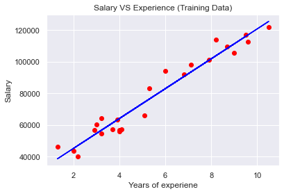
plt.scatter(X_train,y_train,color='red')
plt.plot(X_train,regressor.predict(X_train),color='blue')
plt.title('Salary VS Experience (Training Data)')
plt.xlabel('Years of experiene')
plt.ylabel('Salary')
plt.show()

<matplotlib.collections.PathCollection at 0x170fab89670>

[<matplotlib.lines.Line2D at 0x170fab90700>]

Text(0.5, 1.0, 'Salary VS Experience (Training Data)')

Text(0.5, 0, 'Years of experiene')

Text(0, 0.5, 'Salary')

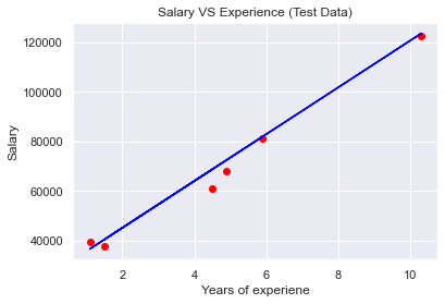
plt.scatter(X_test,y_test,color='red')
plt.plot(X_test,regressor.predict(X_test),color='blue')
plt.title('Salary VS Experience (Test Data)');
plt.xlabel('Years of experiene');
plt.ylabel('Salary');
plt.show()

<matplotlib.collections.PathCollection at 0x170fab2fa60>

[<matplotlib.lines.Line2D at 0x170fab25ee0>]

Text(0.5, 1.0, 'Salary VS Experience (Test Data)')

Text(0.5, 0, 'Years of experiene')

Text(0, 0.5, 'Salary')

Naive Bayes#

from sklearn.datasets import load_iris
from sklearn.model_selection import train_test_split
from sklearn import metrics
from sklearn.naive_bayes import GaussianNB

# Load the data
from sklearn.datasets import load_iris
iris = load_iris()

from matplotlib import pyplot as plt

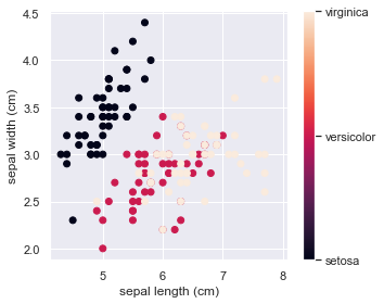
# The indices of the features that we are plotting
x_index = 0
y_index = 1

# this formatter will label the colorbar with the correct target names
formatter = plt.FuncFormatter(lambda i, *args: iris.target_names[int(i)])

plt.figure(figsize=(5, 4))
plt.scatter(iris.data[:, x_index], iris.data[:, y_index], c=iris.target)
plt.colorbar(ticks=[0, 1, 2], format=formatter)
plt.xlabel(iris.feature_names[x_index])
plt.ylabel(iris.feature_names[y_index])

plt.tight_layout()
plt.show()

<Figure size 360x288 with 0 Axes>

<matplotlib.collections.PathCollection at 0x170fab46c10>

<matplotlib.colorbar.Colorbar at 0x170faa3f880>

Text(0.5, 0, 'sepal length (cm)')

Text(0, 0.5, 'sepal width (cm)')

irisdata = load_iris()

print(irisdata.DESCR)

.. _iris_dataset:

Iris plants dataset
--------------------

**Data Set Characteristics:**

    :Number of Instances: 150 (50 in each of three classes)
    :Number of Attributes: 4 numeric, predictive attributes and the class
    :Attribute Information:
        - sepal length in cm
        - sepal width in cm
        - petal length in cm
        - petal width in cm
        - class:
                - Iris-Setosa
                - Iris-Versicolour
                - Iris-Virginica
                
    :Summary Statistics:

    ============== ==== ==== ======= ===== ====================
                    Min  Max   Mean    SD   Class Correlation
    ============== ==== ==== ======= ===== ====================
    sepal length:   4.3  7.9   5.84   0.83    0.7826
    sepal width:    2.0  4.4   3.05   0.43   -0.4194
    petal length:   1.0  6.9   3.76   1.76    0.9490  (high!)
    petal width:    0.1  2.5   1.20   0.76    0.9565  (high!)
    ============== ==== ==== ======= ===== ====================

    :Missing Attribute Values: None
    :Class Distribution: 33.3% for each of 3 classes.
    :Creator: R.A. Fisher
    :Donor: Michael Marshall (MARSHALL%PLU@io.arc.nasa.gov)
    :Date: July, 1988

The famous Iris database, first used by Sir R.A. Fisher. The dataset is taken
from Fisher's paper. Note that it's the same as in R, but not as in the UCI
Machine Learning Repository, which has two wrong data points.

This is perhaps the best known database to be found in the
pattern recognition literature.  Fisher's paper is a classic in the field and
is referenced frequently to this day.  (See Duda & Hart, for example.)  The
data set contains 3 classes of 50 instances each, where each class refers to a
type of iris plant.  One class is linearly separable from the other 2; the
latter are NOT linearly separable from each other.

.. topic:: References

   - Fisher, R.A. "The use of multiple measurements in taxonomic problems"
     Annual Eugenics, 7, Part II, 179-188 (1936); also in "Contributions to
     Mathematical Statistics" (John Wiley, NY, 1950).
   - Duda, R.O., & Hart, P.E. (1973) Pattern Classification and Scene Analysis.
     (Q327.D83) John Wiley & Sons.  ISBN 0-471-22361-1.  See page 218.
   - Dasarathy, B.V. (1980) "Nosing Around the Neighborhood: A New System
     Structure and Classification Rule for Recognition in Partially Exposed
     Environments".  IEEE Transactions on Pattern Analysis and Machine
     Intelligence, Vol. PAMI-2, No. 1, 67-71.
   - Gates, G.W. (1972) "The Reduced Nearest Neighbor Rule".  IEEE Transactions
     on Information Theory, May 1972, 431-433.
   - See also: 1988 MLC Proceedings, 54-64.  Cheeseman et al"s AUTOCLASS II
     conceptual clustering system finds 3 classes in the data.
   - Many, many more ...

irisdata.data

array([[5.1, 3.5, 1.4, 0.2],
       [4.9, 3. , 1.4, 0.2],
       [4.7, 3.2, 1.3, 0.2],
       [4.6, 3.1, 1.5, 0.2],
       [5. , 3.6, 1.4, 0.2],
       [5.4, 3.9, 1.7, 0.4],
       [4.6, 3.4, 1.4, 0.3],
       [5. , 3.4, 1.5, 0.2],
       [4.4, 2.9, 1.4, 0.2],
       [4.9, 3.1, 1.5, 0.1],
       [5.4, 3.7, 1.5, 0.2],
       [4.8, 3.4, 1.6, 0.2],
       [4.8, 3. , 1.4, 0.1],
       [4.3, 3. , 1.1, 0.1],
       [5.8, 4. , 1.2, 0.2],
       [5.7, 4.4, 1.5, 0.4],
       [5.4, 3.9, 1.3, 0.4],
       [5.1, 3.5, 1.4, 0.3],
       [5.7, 3.8, 1.7, 0.3],
       [5.1, 3.8, 1.5, 0.3],
       [5.4, 3.4, 1.7, 0.2],
       [5.1, 3.7, 1.5, 0.4],
       [4.6, 3.6, 1. , 0.2],
       [5.1, 3.3, 1.7, 0.5],
       [4.8, 3.4, 1.9, 0.2],
       [5. , 3. , 1.6, 0.2],
       [5. , 3.4, 1.6, 0.4],
       [5.2, 3.5, 1.5, 0.2],
       [5.2, 3.4, 1.4, 0.2],
       [4.7, 3.2, 1.6, 0.2],
       [4.8, 3.1, 1.6, 0.2],
       [5.4, 3.4, 1.5, 0.4],
       [5.2, 4.1, 1.5, 0.1],
       [5.5, 4.2, 1.4, 0.2],
       [4.9, 3.1, 1.5, 0.2],
       [5. , 3.2, 1.2, 0.2],
       [5.5, 3.5, 1.3, 0.2],
       [4.9, 3.6, 1.4, 0.1],
       [4.4, 3. , 1.3, 0.2],
       [5.1, 3.4, 1.5, 0.2],
       [5. , 3.5, 1.3, 0.3],
       [4.5, 2.3, 1.3, 0.3],
       [4.4, 3.2, 1.3, 0.2],
       [5. , 3.5, 1.6, 0.6],
       [5.1, 3.8, 1.9, 0.4],
       [4.8, 3. , 1.4, 0.3],
       [5.1, 3.8, 1.6, 0.2],
       [4.6, 3.2, 1.4, 0.2],
       [5.3, 3.7, 1.5, 0.2],
       [5. , 3.3, 1.4, 0.2],
       [7. , 3.2, 4.7, 1.4],
       [6.4, 3.2, 4.5, 1.5],
       [6.9, 3.1, 4.9, 1.5],
       [5.5, 2.3, 4. , 1.3],
       [6.5, 2.8, 4.6, 1.5],
       [5.7, 2.8, 4.5, 1.3],
       [6.3, 3.3, 4.7, 1.6],
       [4.9, 2.4, 3.3, 1. ],
       [6.6, 2.9, 4.6, 1.3],
       [5.2, 2.7, 3.9, 1.4],
       [5. , 2. , 3.5, 1. ],
       [5.9, 3. , 4.2, 1.5],
       [6. , 2.2, 4. , 1. ],
       [6.1, 2.9, 4.7, 1.4],
       [5.6, 2.9, 3.6, 1.3],
       [6.7, 3.1, 4.4, 1.4],
       [5.6, 3. , 4.5, 1.5],
       [5.8, 2.7, 4.1, 1. ],
       [6.2, 2.2, 4.5, 1.5],
       [5.6, 2.5, 3.9, 1.1],
       [5.9, 3.2, 4.8, 1.8],
       [6.1, 2.8, 4. , 1.3],
       [6.3, 2.5, 4.9, 1.5],
       [6.1, 2.8, 4.7, 1.2],
       [6.4, 2.9, 4.3, 1.3],
       [6.6, 3. , 4.4, 1.4],
       [6.8, 2.8, 4.8, 1.4],
       [6.7, 3. , 5. , 1.7],
       [6. , 2.9, 4.5, 1.5],
       [5.7, 2.6, 3.5, 1. ],
       [5.5, 2.4, 3.8, 1.1],
       [5.5, 2.4, 3.7, 1. ],
       [5.8, 2.7, 3.9, 1.2],
       [6. , 2.7, 5.1, 1.6],
       [5.4, 3. , 4.5, 1.5],
       [6. , 3.4, 4.5, 1.6],
       [6.7, 3.1, 4.7, 1.5],
       [6.3, 2.3, 4.4, 1.3],
       [5.6, 3. , 4.1, 1.3],
       [5.5, 2.5, 4. , 1.3],
       [5.5, 2.6, 4.4, 1.2],
       [6.1, 3. , 4.6, 1.4],
       [5.8, 2.6, 4. , 1.2],
       [5. , 2.3, 3.3, 1. ],
       [5.6, 2.7, 4.2, 1.3],
       [5.7, 3. , 4.2, 1.2],
       [5.7, 2.9, 4.2, 1.3],
       [6.2, 2.9, 4.3, 1.3],
       [5.1, 2.5, 3. , 1.1],
       [5.7, 2.8, 4.1, 1.3],
       [6.3, 3.3, 6. , 2.5],
       [5.8, 2.7, 5.1, 1.9],
       [7.1, 3. , 5.9, 2.1],
       [6.3, 2.9, 5.6, 1.8],
       [6.5, 3. , 5.8, 2.2],
       [7.6, 3. , 6.6, 2.1],
       [4.9, 2.5, 4.5, 1.7],
       [7.3, 2.9, 6.3, 1.8],
       [6.7, 2.5, 5.8, 1.8],
       [7.2, 3.6, 6.1, 2.5],
       [6.5, 3.2, 5.1, 2. ],
       [6.4, 2.7, 5.3, 1.9],
       [6.8, 3. , 5.5, 2.1],
       [5.7, 2.5, 5. , 2. ],
       [5.8, 2.8, 5.1, 2.4],
       [6.4, 3.2, 5.3, 2.3],
       [6.5, 3. , 5.5, 1.8],
       [7.7, 3.8, 6.7, 2.2],
       [7.7, 2.6, 6.9, 2.3],
       [6. , 2.2, 5. , 1.5],
       [6.9, 3.2, 5.7, 2.3],
       [5.6, 2.8, 4.9, 2. ],
       [7.7, 2.8, 6.7, 2. ],
       [6.3, 2.7, 4.9, 1.8],
       [6.7, 3.3, 5.7, 2.1],
       [7.2, 3.2, 6. , 1.8],
       [6.2, 2.8, 4.8, 1.8],
       [6.1, 3. , 4.9, 1.8],
       [6.4, 2.8, 5.6, 2.1],
       [7.2, 3. , 5.8, 1.6],
       [7.4, 2.8, 6.1, 1.9],
       [7.9, 3.8, 6.4, 2. ],
       [6.4, 2.8, 5.6, 2.2],
       [6.3, 2.8, 5.1, 1.5],
       [6.1, 2.6, 5.6, 1.4],
       [7.7, 3. , 6.1, 2.3],
       [6.3, 3.4, 5.6, 2.4],
       [6.4, 3.1, 5.5, 1.8],
       [6. , 3. , 4.8, 1.8],
       [6.9, 3.1, 5.4, 2.1],
       [6.7, 3.1, 5.6, 2.4],
       [6.9, 3.1, 5.1, 2.3],
       [5.8, 2.7, 5.1, 1.9],
       [6.8, 3.2, 5.9, 2.3],
       [6.7, 3.3, 5.7, 2.5],
       [6.7, 3. , 5.2, 2.3],
       [6.3, 2.5, 5. , 1.9],
       [6.5, 3. , 5.2, 2. ],
       [6.2, 3.4, 5.4, 2.3],
       [5.9, 3. , 5.1, 1.8]])

irisdata.target

array([0, 0, 0, 0, 0, 0, 0, 0, 0, 0, 0, 0, 0, 0, 0, 0, 0, 0, 0, 0, 0, 0,
       0, 0, 0, 0, 0, 0, 0, 0, 0, 0, 0, 0, 0, 0, 0, 0, 0, 0, 0, 0, 0, 0,
       0, 0, 0, 0, 0, 0, 1, 1, 1, 1, 1, 1, 1, 1, 1, 1, 1, 1, 1, 1, 1, 1,
       1, 1, 1, 1, 1, 1, 1, 1, 1, 1, 1, 1, 1, 1, 1, 1, 1, 1, 1, 1, 1, 1,
       1, 1, 1, 1, 1, 1, 1, 1, 1, 1, 1, 1, 2, 2, 2, 2, 2, 2, 2, 2, 2, 2,
       2, 2, 2, 2, 2, 2, 2, 2, 2, 2, 2, 2, 2, 2, 2, 2, 2, 2, 2, 2, 2, 2,
       2, 2, 2, 2, 2, 2, 2, 2, 2, 2, 2, 2, 2, 2, 2, 2, 2, 2])

X = irisdata.data
Y = irisdata.target

X_train, X_test, y_train, y_test=train_test_split(X, Y, test_size=0.2, random_state=0)

gnb = GaussianNB()
gnb.fit(X_train, y_train)

GaussianNB()

y_pred = gnb.predict(X_test)

100*metrics.accuracy_score(y_test, y_pred)

96.66666666666667

# 400 
380 # disease free
20 # disease

380/400

0.95

y_test

array([2, 1, 0, 2, 0, 2, 0, 1, 1, 1, 2, 1, 1, 1, 1, 0, 1, 1, 0, 0, 2, 1,
       0, 0, 2, 0, 0, 1, 1, 0])

y_pred

array([2, 1, 0, 2, 0, 2, 0, 1, 1, 1, 1, 1, 1, 1, 1, 0, 1, 1, 0, 0, 2, 1,
       0, 0, 2, 0, 0, 1, 1, 0])

EAS503

Part 1

Contents

Part 1#

Load sample dataset#

Loading data from the web#

Generate dataset#

Load data from openml.org #

5.3. Preprocessing data#

Standardization, or mean removal and variance scaling#

Can save scaling and apply to testing data#

Scaling features to a range#

Pre-processing data - Non-linear transformation#

5.3.3. Normalization#

Can save the normalization for future use#

Preprocessing data - Encoding#

5.3.5. Discretization#

5.4.2. Univariate feature imputation#

Splitting data into Train and Test#

Linear Regression#

Naive Bayes#

EAS503

Part 1

Contents

Part 1#

Load sample dataset#

Loading data from the web#

Generate dataset#

Load data from openml.org#

5.3. Preprocessing data#

Standardization, or mean removal and variance scaling#

Can save scaling and apply to testing data#

Scaling features to a range#

Pre-processing data - Non-linear transformation#

5.3.3. Normalization#

Can save the normalization for future use#

Preprocessing data - Encoding#

5.3.5. Discretization#

5.4.2. Univariate feature imputation#

Splitting data into Train and Test#

Linear Regression#

Naive Bayes#

Load data from openml.org #